Citation:
Colantuono, G and Kor, A and Pattinson, C and Gorse, C (2018) PV with multiple storage as function
of geolocation to reduce peak demand. Solar Energy, 165. pp. 217-232. ISSN 0038-092X DOI:
https://doi.org/10.1016/j.solener.2018.03.020
Link to Leeds Beckett Repository record:
http://eprints.leedsbeckett.ac.uk/4707/
Document Version:
Article
Creative Commons: Attribution-Noncommercial-No Derivative Works 4.0
The aim of the Leeds Beckett Repository is to provide open access to our research, as required by
funder policies and permitted by publishers and copyright law.
The Leeds Beckett repository holds a wide range of publications, each of which has been
checked for copyright and the relevant embargo period has been applied by the Research Services
team.
We operate on a standard take-down policy.
If you are the author or publisher of an output
and you would like it removed from the repository, please
contact us
and we will investigate on a
case-by-case basis.
PV with multiple storage as function of geolocation to
reduce peak demand
Giuseppe Colantuono, Ah-Lian Kor, Colin Pattinson, Chris Gorse
Leeds Sustainability Institute, Leeds Beckett University, LS1 3HE Leeds, UK
Abstract
A system, modeled in two geolocations (Oxford, England; San Diego, Califor-nia), consists of a PV array and two storage solutions (defined by distinct sets of efficiencies/costs): short term (batteryB) and long term (H, hydrogen reservoir with electrolyzer/fuel cell). The system meets a 1-year, real domestic demand totaling 5 MWh/year. First, it is configured as standalone (SA); then, as grid-connected (GC), receiving 50% of the yearly integrated demand. H and PV are dynamically sized as function of geolocation,B size andH efficiency.
With a 10 kWh battery and a 0.4H cycle efficiency, requiredH capacity for the SA case is∼1230 kWh in Oxford and∼750 kWh in San Diego (respectively, ∼830 kWh and∼600 kWh in the GC case). Related array sizes are, respectively, 93% and 51% of the local reference 8 kWp system (51% and 28% in the GC case). A trade-off between PV size and battery capacity exists: the former grows significantly asB shrinks below 10 kWh. On the other hand, PV size is insensitive to rising B above ∼10 kWh, a capacity large enough to cope with short timescales.
With current PV and B costs, a SA system in Oxford (San Diego) can stay within 104 $ CapEx if H’s cost does not exceed 4 $/kWh (8 $/kWh); these figures increase to 7$/kWh (10 $/kWh) with grid constantly/randomly
supplying a half of yearly energy.
Extending modeling over 18 years makes results varying to different extents, depending on location; in any case, less than±10% of the reference year.
Keywords: electricity storage, energy meteorology, solar energy, load following, power grid
1. Introduction
Non-constant output is a major obstacle towards a widespread exploitation of wind and solar photovoltaic (PV) generation, and a risk factor for the op-erational integrity of power distribution networks (Boyle, 2012; Steinke et al.,
grid, and to cope with demand drops caused by PV domestic installations’ out-put during sunny days (Denholm et al., 2015). Storage on the users’ side can also free the grid from the need of following demand. The price of batteries was still relatively high at the beginning of the 2010s (Mulder et al.,2013;Juul,
2012) but has then started to decline sharply; by some analysts (Hensley et al.,
2012), this decreasing trend is projected to continue.
PV power is a typical example of highly inconstant renewable generation. Time-variability of solar irradiance on the Earth surface is due to two main astronomical facts, Earth rotation and revolution, which in turn correspond to separated timescales: day-night and seasonal cycles. The third source of ir-regularity is due to weather and climate, and is superimposed to the purely deterministic astronomical oscillations. It is often termed as intermittency in renewables literature and has a prominent effect on PV output, particularly in cloudy regions (see for exampleColantuono et al.,2014a). Energy meteorology (Emeis,2012;Kleissl,2013;Olsson,1994) is a growing field of research and testi-fies the importance of environmental analysis for maximizing renewables’ output and quantifying/reducing uncertainty (Correia et al.,2017;Prasad et al.,2015;
Colantuono et al.,2014b).
Storage coupled to PV power must therefore cope with these three sources of output variance. Other more or less unpredictable local factors that can fur-ther affect PV output range from module uncleanliness (Mani and Pillai,2010), age-induced degradation (Kaplanis and Kaplani, 2011) and failure, to build-ings obstructing the horizon (Erd´elyi et al.,2014) and tree growth (Dereli et al.,
2013). Domestic electricity demand is also affected by the discussed variability, as lighting and heating needs depend on season and weather patterns. All these environmental factors reach prominent importance when renewables supply a relevant fraction of electricity, because they affect both the generation and the demand side. PV is the only renewable source widely used on the domestic side, or for otherwise “small” applications (“microgeneration”: typically, few kWp, kWh of rated power, or less). From the distribution point of view, microgen-eration reduces the customer’s demand (before any residual is uploaded to the grid), while other renewables are integrated in the distribution network. The present model requires microgeneration be used locally: first, in a standalone (SA) configuration, and then in a grid-connected (GC) one.
locations by the requirement of matching the same domestic load’s yearly time-series. PV size is expressed by means of the scaling factor X, the fraction of the size of an 8 kWp array used as reference. The partition of storage into a long-term reservoir and a short-term, more efficient and smaller one is justified if a trade-off between storage cost and conversion inefficiency is possible.
Current storage technologies possess various efficiency levels; here, hydrogen H and batteryBare characterized by their round-trip efficiency values ηH and
ηB. Hefficiency is given three values: ηH= 30%, 40% and 50%, a range similar to what reported inLuo et al.(2015, Table 11 therein), while the battery efficiency is fixed at ηB= 85% (ibid.). The latter value can fall either within the lithium-ion (Rastler, 2010) or the Lead-acid (Beaudin et al.,2010) efficiency interval. The smallest ηH value is the closest to the currently available electrolysis/fuel-cell cycle; significant improvements may be expected with standardization and mass production, as hydrogen storage is still in the development phase (Luo et al.,
2015).
PV generation is then supplemented by a power grid able to provide only constant power. This scenario is aimed at exploring storage as a substitute of the current load-following pattern (e.g. Mosh¨ovel et al., 2015); the amount of long- and short-term storage needed on the user’s side to accommodate such a constant supply is quantified. This idea is further extended that a partly random power provision is fed by utilities to domestic customers, to understand how user’s storage may cope with a grid that, besides not following demand, does not mitigate the variability on the supply side induced, for example, by wind and solar farms.
The two compared geographical locations are Oxford in the South of Great Britain and San Diego in Southern California. PV output and states of charge of the storage reservoirs are expressed as function of time in the two geolocations; PV arrays’ sizes and reservoirs’ capacities are determined in each location for a number of system configurations. Engineering implementation is beyond the scope of this analysis, the focus of which is energy balance. Exactly matching storage to given yearly demand and PV generation timeseries is not sufficient to size a real system, due to year-to-year variability. Further analysis is there-fore performed to understand the behavior over many years, with the resulting variations of required generation and storage capacity.
2. Modeling the system
2.1. Generalities
losses due to storage round-trip conversions are taken into account. This im-plies that changingB reservoir’s size makes PV array’s area andH’s capacity changing as well. Further case studies include power provision from the electric grid in the amount of 50% of the yearly-integrated demand, with PV array’s size reduced accordingly.
Table 1: Main symbols
Symbol Definition
S() Heaviside’s step function
T = 1 yr Length of the problem in time
0≡t0, t1, ...tn, ..., tN≡T /t1 60 s time-steps;N= T /60s≡525600
dB Power drawn from battery
dH Power fromH to battery
uB Power fed to battery
uH Power fed toH
λ Electric power load in kW
γ PV power generation
δ Difference between generation and demand
X Fraction of the reference, 8 kWp PV array
B Battery (and its state of charge)
H Hydrogen storage (and its state of charge) ηH Energy efficiency of long term storage (H) ηB Efficiency of short term storage (battery)
Bm Minimum battery charge level
BM Battery capacity
A system with no battery (endowed withH only) has not been considered due to the relatively slow start-up time of fuel cells. Battery is never discharged belowX·max(λ)∗600 s = 0.91·X kWh, where X is the PV array scale factor in terms of percentage of the reference, 8 kWp array; a 600 s interval is of the order ofH’s reservoir latency. Such a buffer should ensure power shortage avoidance; it also causes effectiveBcapacity to be lower than labeled. In a real system, an additional small penalty, neglected here, would be present, because a fraction of the power drawn fromH would be routed through B in transient phases, between the timeH kicks-in until it reaches working conditions. The number of such transients would be relatively small, asH tends to be switched on/off with a much lower frequency with respect to battery.
2.2. Governing equations
We are aimed at determining storage reservoirs’ states of charge B(tn) and
H(tn) as function of previous states B(tn−1) and H(tn−1) and of generation
henceforth omitted to simplify notation, barring cases where functions depend on previous time step tn−1.
We first define δ, the difference between generation and load at any timetn:
δ = X·γ − λ; (1)
X scales the generation timeseries γ to adapt PV array’s nominal power to system’s features as they are varied throughout the model’s scenarios.
We then label uploaded and downloaded power as uX and dX.
Conse-quently, the non-negative variables uB and uH quantify the power uploaded to
batteryB and to long-term reservoir H, respectively:
uB =S[BM −η
Bδ−B(tn−1)]· S(δ)·δ+
+ S
−[BM−ηBδ−B(tn−1)] ·[BM−B(tn−1)]/ηB, (2)
uH =S−[BM −η
Bδ−B(tn−1)] ·
δ+ [B(tn−1)−BM]/ηB ; (3)
symbols are detailed in Table1, while
S(x) =
(
1, if x >0 ; 0, otherwise
is the Heaviside’s step function according to the S(0) = 0 convention (brackets of any kind following S always denote its functional argument). This function plays the role of a switch, defining the system’s regime: for example, when δ changes from positive to negative, the quantity S(δ) goes from 1 to zero, setting the first term of Eq. (2) to zero. This is all the more so for the second term (and for the right-hand side of Eq. 3 as well), because δ≤0 implies ηB·δ+B(tn−1)−BM ≤0.
Battery is being charged (uB>0 ) when both generation is larger than λ
(that is, δ >0 ) and B is not full; if either condition is not met, uB= 0 holds
instead. On the other hand, long-term storageHis being charged (uH>0 ) when
δ >0 and B is completely filled up; that is, the relationships B(tn−1) =BM
and X·γ > λ are true at the same time. The first term of Eq. (2) represents the case in which the 60 s “energy packet” to be loaded at the current time-step does not saturate the capacity of the battery when added to the energy already in it. The second term refers to the incoming packet saturating the battery, in which case the packet can only be partially taken up. In the latter instance, the energy uploaded toB corresponds to the difference between capacity BM
and B(tn−1), the level of charge resulting from balance at previous time-step.
Power downloaded from reservoirs is instead denoted by the non-negative functions dB and dH:
dB = − S(−δ)·δ; (4)
dH = − S(−δ)· S[Bm−B(tn
−1)]·δ; (5)
that is, the common, necessary condition for dB and dH to differ from zero is
X·γ < λ. dB also needs to satisfy Bm≤B(tn
−1)≤BM (the Heaviside’s condition
expressing the latter inequality is automatically satisfied and therefore absent from Eq.5); dH must meet B(tn
−1)< Bm instead.
The drop of battery level below the threshold value Bm is the event that
triggersH’s discharge (Eq.5): as soon as the quantity Bm−B(tn−1) becomes
greater than zero, H starts to provide an amount of energy equal to |δ| that, added to generation, satisfies demand. Battery level is restored at B=Bm or
higher as soon as δ becomes greater than zero. Until that occurs,H remains active; that is,dH remains above zero.
We can finally quantify the energy level in bothB andH reservoirs:
B =S(t2−tn)·BM + S(tn−t1)·B(tn−1) + ηBuB +dH −dB ; (6)
H =S(t2−tn)·H(0) +S(tn−t1)·[H(tn−1) +ηHu
H −dH] ; (7)
Heaviside’s conditions, in this case, separate reservoirs’ initial energy level (tn=
1) from the evolution that follows (tn>1).
In summary, both B and H depend on load λ and generation Xγ via δ through Eqs. (2-4); B andHalso depend on time, on the fixed parameters Bm,
BM, ηB, ηH, and on their prior states. Examples of the behavior of the seven
variables defined by Eqs. (1-7) are displayed inAppendix B.
The energy in the dH term is recorded as “in transit” through the battery
(penultimate monomial in Eq.6) to stress that it is battery’s sub-threshold level that triggers and keeps H’s discharging. However, dH is thought to bypass
B and satisfy demand without any intervening stage (keeping in mind what discussed on H’s transients at bottom of Section 2.1): the ηB energy penalty is therefore not assigned to dH. Real-world systems could clearly be tweaked
with different criteria; the implementations of these range of conditions will be use cases. The present implementation, which minimizes the required PV array size by using the less efficient, long-term reservoir only when battery is full, has the advantage of not requiring any kind of online computation.
The last equation needed to close the problem is given by the constraint
H(T) + B(T) = H(0) +BM. (8)
The requirement that the amount of long-term stored power at the end of the yearly period equals the initial level (system is set to start with a full battery, implying B(0)≡BM in Eq. 8) assures that yearly-integrated generation and
Eq. (8) will be considered satisfied if the two sides differ less than a predeter-mined amount (“error”).
Once B’s capacity is fixed and both H and the PV array are sized accord-ingly, the historical data (past generation and demand timeseries) will not be necessary for operating a real system. The approach here is aimed at high-lighting geographical/climate differences, and the behavior induced by various battery sizes. The sizing of a real system would have to account, for exam-ple, for year-to-year differences in solar generation and electricity consumption, failure rate, and other unpredictable factors; consequently, some form of un-certainty evaluation should be introduced, e.g. loss-of-load probability (LOLP, discussed by Celik, 2007; Klein and Beckman, 1987; Schenk et al., 1984, and many others). The impact of differences in PV generation over many years is addressed in Section 5, as well as the effect of varying demand. LOLP esti-mation is not addressed here, as it would not make substantial contribution to frame the problem of multiple storage as function of climate and geolocation.
2.3. Solution of Eqs (1-8)
Equations are solved for every time tn as function of previous time tn−1,
for a guessed value of X; the procedure is being iterated until “error” falls below a predetermined threshold. H at t= 0 contains an amount of energy equal to 2 months of the yearly integrated load: H(0) = (5/6) MWh (the used datasets are detailed in the next section). The first step (from 00:00 to 00:01, January 1) simply updates battery storage, which is being depleted by 60 s worth of load as PV generation is zero at nighttime. As time advances, the appropriate Heaviside’s functions will transit from zero to 1 and vice versa. B becomes progressively depleted, but the Sun later kicks in. B may therefore be recharged or, if generation is insufficient, may fall below the minimum levelBm,
in which caseH will start to feed the demand instead. At the end of the yearly timeseries, the final valueH(T)+B(T) is recorded.
For the sake of computing a practical solution, Eq.(8) is replaced by the following approximate condition, as anticipated above:
|H(T) + B(T) −H(0) −BM| < 10 kWh. (9)
If Eq. (9) is not satisfied and the argument of the absolute value on the left-hand side is negative, the size of the PV array is increased by increasing X; if, on the contrary, such an argument is positive, X will be reduced. After this update the procedure is repeated andH updated again. The process is interrupted as soon as the condition in Eq. (9) is met. Capacity of long-term storage H is defined as
H = max [H(tn)] −min [H(tn)]. (10)
keep the model running and the iterations following one another until an ap-propriate PV array’s size is found and the inequality at Eq. (9) satisfied. When this occurs, yearly generation balances the yearly demand, storage’s round-trip penalties included.
2.4. Demand and Generation data
A domestic consumption timeseries and a PV generation one are needed in each geolocation in order to address the formulated problem. the same domestic-load timeseries (Lichman,2013) is used in both localities: Oxford, UK (hereafter Oxford,Oxford PV array 2016) and San Diego, CA, USA (hereafter San Diego,
PVOutput.org 2017b). This choice has the downside of neglecting the local correlation between PV generation and household power demand (e.g., on a sunnier-than-average day, lower lighting demand may be expected, together with relatively high PV output) but has the big advantage of comparing the performance of both generation and storage in different locations against the same demand curve, which is the main goal of this study. With the loss of co-spatiality between generation and demand, contemporaneity loses its meaning, too: timeseries have been therefore chosen to prioritize availability and data integrity.
The load λ is normalized to 5 MWh of yearly generation, which cuts ap-proximately by a half the original load’s size. This integrated value is consid-erably lower than the average electrified USA home (∼ 12300 kWh in 2014,
Energy Efficiency Indicators 2016) but higher than the yearly consumption of the average electrified home in the European Union in the same year (∼3600 kWh, ibid.) and in China (∼1600 kWh).
As already specified, the PV scaling factor X expresses the size of the needed PV array as a fraction of the reference 8 kWp PV array. The PV size needed in San Diego to achieve Oxford’s output is 61% of Oxford’s array, for the yearly timeseries used (Appendix A). This clearly introduces a dependency on the particular year considered when comparing the two geolocations. In Section5, 18-year long records are considered, to overcome this limitation and to determine a range of variability for the model’s quantities in both places. The size of PV arrays is expressed in kWp, to keep our conclusions with the highest possible independence on the technology used. The two arrays have diverse orientations; none of the azimuths is due south (see Appendix A), meaning that the two PV arrays are surely sub-optimal. This does not diminish the significance of the present analysis because climate differences are overwhelming and the differences induced by systems’ configuration (battery size, H efficiency, grid supply) are assessed by comparing results locally. Last but not least, orientation is rarely optimal for real, domestic PV arrays (usually constrained by the existing built environment,Colantuono et al. 2014a) and often known/reported by the owner with significant approximation (ibid.).
3. Results
3.1. Standalone systems
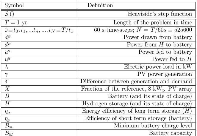
[image:10.612.132.481.269.420.2]Standalone systems are useful analysis targets not only per se; they can be viewed as the limiting case for grid-connected (GC) systems, with microgenera-tion and storage, as grid-supplied electricity is progressively reduced. Eqs. (6-8) are solved forB,H, and X thirty times for each location, in order to combine three values of ηH (0.3, 0.4, 0.5) with ten values of battery size (2 to 20 kWh with 2 kWh increment). Solutions are sought by dynamically adjusting X such that X·γ satisfies the demand λ (Lichman,2013) for the chosen battery size within the specified, 10 kWp error.
Figure 1: PanelA. Curves represent long-term storageH throughout the year. H’s round-trip efficiency ηH (the second field in the legend, after geolocation) is being parametrically varied. The third field represents X, the PV array scaling factor; a similar scaling coefficient applies if PV’s area is considered instead of peak power, provided technology is the same for all systems. The high degree of similarity at large-scale, between curves representing very different battery sizes in the same geolocation, may be misleading; a zoom on small scales features of the curves (Fig.4) shoes the small-scales differences between systems with large and small batteries. Oxford’s and San Diego’s bunches of curves are well separated; they can be represented with the same line styles.H’s curves in Oxford (San Diego) boast higher (lower) maxima and lower (higher) minima: more energy must be stored in Spring/Summer (Summer from now on) to be used in Fall/Winter (hereafter Winter) in more poleward latitudes. Battery has capacity BM= 10 kWh. PanelB. Standalone (SA) systems compared to grid-connected
(GC) ones, supplied with constant power summing up to 50% of integrated yearly demand, for the intermediateηH= 0.4 value. GC case with 25% of random-varying power is not plotted as virtually indistinguishable from the constant-power case. Required long-term storage capacity in Oxford (San Diego) falls from∼1230 KWh to∼830 KWh (∼750 KWh to∼600 KWh) with
constant grid supply; capacities are the same for GC case with random-component).
efficiency ηH between 30% and 50% and a 10 kWp battery. The same conditions in Oxford require an array ranging from 85% to 105% of the 8 kWp reference power. The required PV size decreases with increasing ηH because a more ef-ficient H storage reduces conversion losses and, consequently, the generation which is required to match demand. On the other hand, the required H ca-pacity grows as a smaller PV array increases the need of storing energy from Spring/Summer (Summer from now on) to Fall/Winter (Winter from now on). In other terms, with a larger PV array and a less efficient seasonal storageH, more power is proportionally wasted in Summer to load the hydrogen reservoir (it is useful to recall that round-trip inefficiencies are here computed at once when energy is uploaded to reservoirs) but less energy is actually uploaded, as the larger array is closer to self-sufficiency in winter. Unlike Fig. 1A, where
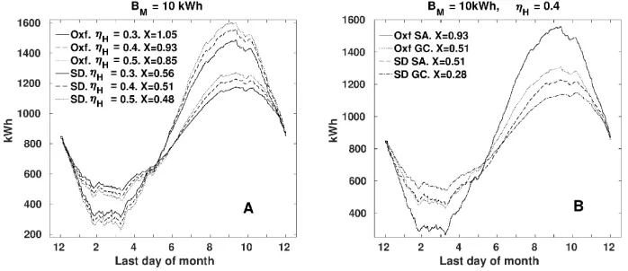
Figure 2: Panel A. Like Fig. 1A, with battery capacity being parametrically varied. As in Fig.1A, the three San Diego curves reflect a much lower seasonal variability and are well separated from Oxford’s ones. Legend’s fields indicate geolocation,Bcapacity and PV array’sscaling factor X; such a value needs to be multiplied by 8 kWp, the array’s reference
size. Long-term storage round-trip conversion efficiency is here set toηH= 0.5, the highest value. PanelB. Systems are compared from an alternative point of view, which highlights the different usage of long-term storage when geolocation and ηH are varied: “roughness”
r (Eq. 11) is depicted. Higher r values indicate higher reliance onH and a “rough”H’s profile (Fig.4): the long-term reservoir’s usage is proportionally higher on short timescales.
r is inversely related to battery size, and is higher in the poleward location.
difference in the PV array size required by B= 2 kWh and B≥10 kWh suggests that the separation between long-term (seasonal) and short-term (daily-hourly) storage arises in a seamless and “natural” way when battery is large enough. No energy-management algorithm is required to direct power to the appropriate reservoir: the simple rule of first fillingB up to capacity, and only subsequently converting electricity to hydrogen and loading theH reservoir, has the property of minimizing conversion inefficiencies and therefore minimizing the PV area required to feed the system.
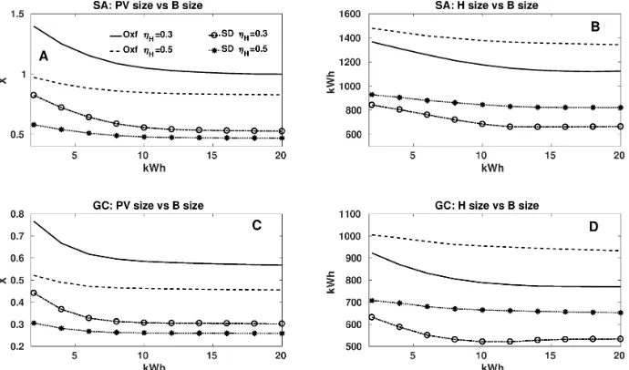
[image:12.612.135.480.327.530.2]The impact of battery size on PV size is further clarified by Fig.3 (which also shows the similar effect battery size has on required H capacity): in both locations, for the same demand timeseries totaling 5 MWh per year, the 10 kWp value can be loosely seen as the boundary between a capacity range (B.10 kWh) characterized by a relatively strong dependency between battery capacity and PV size, and a range (B&10 kWh) where such a dependency is noticeably weaker as added battery capacity improves system’s efficiency only marginally.
Figure 3: Panel A. PV array size as function of battery size in the two geolocations, for different values of hydrogen round-trip conversion efficiency. PanelB. Required capacity of the hydrogen reservoir as function of battery size in the two geolocations, for the same values of hydrogen conversion efficiency considered in PanelA. PanelsC-Dare like PanelsA-Bfor the grid-connected (GC) case (Section3.2). Legend in PanelArefers to all plots.
Figure2B depicts the “roughness” parameter, defined as
r =
Z T
0
dH(t) dt
dt , (11)
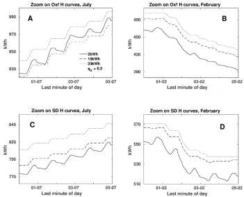
of battery usage: from sub-hourly to daily. Sensitivity of r to battery size, hydrogen round-trip efficiency and geolocation can be inferred from Fig. 2B: r combines the main three factors that determine the “amount of activity” of long-term storageH. Figure2B also shows how roughness r is inversely propor-tional to ηH; while this result can be counterintuitive, it is physically justified because the system with more efficient long-term storage needs a smaller PV array (Fig.1A), as a smaller amount of energy needs to be uploaded for winter months. This, in turn, implies that reliance on storage is on average higher on a daily basis; the fraction of energy “improperly” uploaded to/downloaded from theH reservoir at small timescales is consequently higher as well. Figure4, by means of zooming on small-scale features ofH’s curves in Winter and Summer, provides a pictorial justification for r trends. Small batteries cause the usage ofH for daily storage, as the pronounced local minima of the B= 2 kWh curves suggest.
3.2. Grid-connected systems
GC systems’ behavior is analyzed and compared to the SA cases in two different configurations. We first postulate a grid providing a constant supply throughout the whole period, equal to 50% of the 5 MW yearly integrated load; this choice leaves to storage the burden of following demand. In the second case the given load is satisfied in both geolocations with the aid of a grid that, although still providing 50% of yearly-integrated load, is freed from the constancy constraint: power provision can oscillate randomly in time between 25% and 75% of the average demand; that is, between 143 W and 428 W.
The latter instance may exemplify a grid delivering power from intermittent sources like wind farms or solar farms: domestic storage is not only used to regularize locally generated power, but to allow the grid to deliver variable power according to instantaneous production. Similarly to what pointed out for the SA system (Section3.1), the modeling strategy maximizes energy efficiency and therefore minimizes PV size for the given load (and for the given grid timeseries, in the random case). It will be shown in Section5 that random permutations in hourly load produce undetectable changes in the ensuing system’s size.
Figure 4: 5-day zooms on the curves of Fig.2A, highlighting small-structure differences in-duced by battery size. A smallerBforces the system to “improperly” use long-term storage
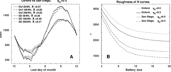
H for daily and sub-daily transactions. In Summer (PanelsA,C), the curves are increasing on a sufficiently large timescale (>1 day), as energy is being stored for the following Winter. Local minima (troughs) for the case of smallest battery (2 kWh) denote usage ofHat short timescales. Larger batteries instead (dashed and dotted line) forceH to follow a Summer “staircase pattern”, with the hydrogen reservoir charging up in daylight and idling at night-time. Pronounced local minima are also present in California in February in the small-battery case, because generation at that time of the year is already sufficient to store a significant amount energy from day to night. Legend in PanelAand H’s efficiency refer to all plots. FiguresB.8-B.11inAppendix Bdisplay PV generation (bottom right Panels) for the initial two days of both 5-day periods
4. Simple CapEx analysis
The total, one-off capital cost (CapEx) of the system is examined as a func-tion of geolocafunc-tion and ofH’s CapEx, and in relation to the other parameters that determine system’s size. The economical analysis is limited to CapEx be-cause uncertainties on long-term storage’s standards and future technical devel-opments make detailed financial estimates difficult: for example, a gas storage tank may potentially last for an arbitrary long time while other components (fuel cells, electrolyzer) do not (Schmittinger and Vahidi, 2008; Carmo et al.,
at approximately the modules’ midlife (Colantuono et al.,2014a), while battery duration depends on frequency and depth of discharges (Divya and Østergaard,
2009).
Even if we limit the analysis to CapEx, H’s cost remains highly uncertain: neither adequate hydrogen storage facilities have been deployed so far, particu-larly for domestic use, nor unified technical standards exist. Economy of scale has the potential for causing a massive cost reduction, in line with what hap-pened for decades with PV modules (International Renewable Energy Agency,
2015) and batteries (Hensley et al.,2012). Cost reduction can also be achieved by means of sharing facilities across multiple homes, which could carry the addi-tional benefit of reducing the total required capacity. The electrolysis/fuel cells cycle is chosen in this work, but other strategies are not ruled out asH storage is here defined by round-trip efficiency, ηH, and unitary cost only. Fuel cells market price is currently around 2000$/kW (Crow and Johnston,2016), while
electrolyzers have been reported to be around 1000$/kW byPenev(2013), who
also estimated the reservoir’s CapEx at 2.5 $/kW in the cheapest case (liquid
hydrogen, in which case CapEx and energy expenditure for a compressor should be factored in) for large installations. 1 kW electrolyzer could suffice for coping with a load totaling 5 MWh/year; this would, however, require an extra battery to buffer the energy to be uploaded toH in instances of generation exceeding load by more than 1 kW (δ > 1 kW), because B is full to capacity whenever H starts to be loaded. A similar mechanism would hold for fuel cells and the energy to be downloaded as soon asBhas been depleted. The presence of such an extra battery would introduce a trade-off between its size and efficiency and fuel cells’/electrolyzer’s capacities/costs, similar to the balance analyzed in this work between PV array’s size/cost and battery’s size/cost.
Given the large indetermination on so many factors, we let ample varia-tion of H’s CapEx , with the basic goal of determining a target range for it through the resulting CapEx of the whole system: H’s CapEx is therefore al-lowed to vary between 0.1 $/kWh and 70 $/kWh. The picked cost of PV
array is 3000$/kWp instead, while the chosen cost of batteries is 227 $/kWh
(Hensley et al., 2012).
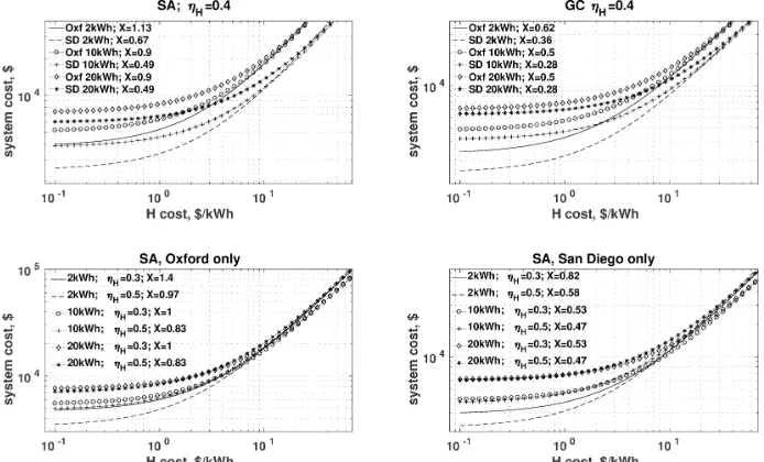
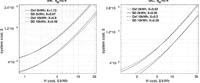
Figures 5-6 summarize CapEx analysis. The first feature to be noticed is that, for inexpensive H, the cost curves “cluster” mainly due to B size; for expensive H, they depend more markedly on geolocation instead (Fig. 5A-B). When long-term storage is on the expensive end,H’s required capacity becomes the main CapEx discriminator, meaning that the influence of geolocation on system’s cost increases: Oxford’s large seasonal differences in PV output require a larger amount of seasonal storage with respect to San Diego (Fig. 5A-B). The amount of long-term storage is not significantly influenced by battery size. A small battery forces the system to use seasonal storage inefficiently, on a daily/sub-daily basis (as shown by the plot of roughness r, Fig.2B); however, the capacity used for such fast transactions is negligible (∼10 kWh) and does not significantly affect the capacity involved in seasonal storage, which is of the order of 1 MWh.
Figure 5: Summary of cost analysis. Xrepresents the size of the PV array;X= 1 corresponds to an 8 kWp array.
costs in the two geolocations does not change much as function of H cost, either with grid or without; moreover, no detectable difference exists between the case of a constant supply fed to the system and the case of a half of the integrated supply randomly varying. For negligibleH’s CapEx, higher Oxford’s cost is due to larger PV array; as long-term storage gets more expensive and gradually becomes the main factor in determining system’s cost, Oxford remains more expensive due to the much more pronounced irradiance seasonal imbalance which dictates an increase inH capacity.
Figure 5C (Oxford) and Fig.5D (San Diego) reveal the influence of ηH on system’s cost. When battery is large, a significant variation in ηH has a small impact on the system cost. With a smaller battery, on the contrary, variations in ηH are noticeable due to the increased usage of long term storage at high frequencies (daily and sub-daily) which, in turn, imposes a larger and more costly PV array. System’s qualitative behavior in San Diego is very similar to Oxford in this respect, except for a generally higher cost in the more poleward location.
It may be also worth commenting on the cap that needs to be imposed on H cost in order to keep system’s CapEx below a given threshold, say 104$. For SA systems, ηH = 0.4 (Fig. 5A), H’s CapEx is around 4$/kWh in Oxford in
combination with a 10 kWh battery, which increases by some tenths of$/kWh
in the same location if the battery is 2 kWh. The equivalent figures in San Diego are almost identical and higher, ∼8 $/kWh, because of the lower need
104$for a higherH cost in every situation: respectively,∼7$/kWh in Oxford and more than 10$/kWh in San Diego for both battery sizes. A larger battery,
10 kWh or more, becomes competitive at higher systems’ costs, around 2×10⁴$ for the SA,ηH= 0.4 case (Fig.5A). It should be kept in mind that the 2 kWh battery asks for a PV array ∼20% larger than what needed by the 10 kWh battery; the 1.13×8 kWp array required in Oxford in the smallest battery’s case (Fig.5A) corresponds to an area around 45 m2with current modules’ conversion rate, which become more than 65 m2 for η
H = 0.3 (Fig.5D); this figure could
grow larger in case of disadvantaged PV layouts, often constrained by the built environment (Colantuono et al., 2014a). The chance of reducing PV modules’ area may introduce savings or prevent additional penalties not quantified in the present calculation. This trade-off between battery capacity and PV array’s area appears to be a key feature in densely populated areas with tall buildings. As already noticed, long-term storage dominates system’s CapEx when more expensive than a few $: partly because a smaller (larger) battery requiring a
larger (smaller) PV array implies these system’s components partially balance each other out. The other reason is the large required capacity for seasonal storage, particularly in the poleward location. Reasonably priced long term storage appears therefore as a key condition for making SA systems viable or for allowing power grids to deliver constant or even “arbitrary” power throughout the year. As a further test, Fig.6 reports CapEx behavior when battery cost is reduced by a factor 3, from 227 $/kWh down to 76 $/kWh; the larger battery becomes slightly economically convenient between 1 and 11$/kWh in the four
[image:17.612.134.480.424.568.2]cases.
5. Varying demand timeseries. Extending PV generation to multiple years. Implications for system sizing
Analyzed generation and demand timeseries are 1 year-long, mainly due to data availability. In order to generalize results, we hereby show the implications of varying λ demand timeseries and considering multiple years of PV output.
λ periodicity is 60 s; in order to test sensitivity to demand’s alterations, the 365×24 hours in the 1 year time interval have been randomly permuted 120 times for various parameter combinations; in all cases, the change of PV size necessary to cope with the modified load is much smaller than 1% and within the model error, which is dictated by the 10 kWh tolerance (Eq. 9) in the approximate solutions of the model equations. Similarly, the behavior of H(tn) (the graph
of which is exemplified in Figs.1and 2A) remains practically unchanged after hours’ permutations. Recalling the definition of δ (Table1), random changes of generation γ have an effect which is similar to random variations of λ. This suggests that random generation/demand permutations do not significantly alter energy balance and system components’ sizes.
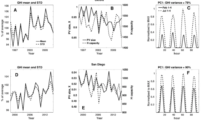
Many years of PV generation need then to be considered in both geoloca-tions, to generalize the model output and, particularly, PV array size andH’s re-quired capacity. Given the short length of the analyzed PV output, the authors turned their attention to global horizontal irradiance (GHI) timeseries spanning much longer intervals. A GHI measurement station has been chosen within 100 km of the PV location in Oxford (UK Meteorological Office 2013, station ID 461, ∼52.23oN, ∼0.46oW) and San Diego (National Solar Radiation Database
2015, station ID 210008, ∼32.73oN, ∼117.14oW); timeseries are 18 year-long (1995-2012 in Oxford; 1998-2015 in San Diego) with half-hourly/hourly (Ox-ford/San Diego) sampling period.
The goal is to create yearly PV generation timeseries that are, from the climate and geographical standpoint, analogous to the available ones, with 60 s sampling period. Every GHI yearly record is first normalized to the available, local yearly PV generation record. Subsequently, the local sub-hourly PV vari-ability (obtained by subtracting the local hourly means) is linearly superimposed to the normalized GHI timeseries. Finally, the 18 yearly GHI records in each location are once more individually rescaled, this time to restore the relative, year-to-year average disparities. This way, 18 years of PV “pseudo-generation” timeseries are obtained in both locations from real GHI timeseries and used as the model input to asses the year-to-year variations in the required PV size and H’s capacity (Fig.7B,E). With the data-procedure just outlined, the reference year’s record of PV generation used so far (in both Oxford and San Diego), integrated in time, constitutes by construction the average of the 18 years of pseudo-generation.
Figure 7: PanelsA,Ddisplay GHI (kW/m2) over the entire interval. PanelsB,Eshow PV
size and H capacity during 18 model runs per geolocation using PV “pseudo-generation” as input, obtained from the 18-year GHI records as described in the main text. Required storage’s and PV’s size variability from year to year is portrayed. In PanelsC,Fthe first principal component (PC1) of the 18 yearly timeseries is plotted for a few Winter and Summer days. PC1 accounts for the day-night cycle (crests and troughs with 24 hr period) and for the seasonal cycle (greater magnitude of Summer/dashed curves’ peaks with respect to solid curves’ peaks). PC1 is associated to 78% of variance in Oxford and to 90% of variance in San Diego; each higher order PCs explains less than 2% of variance in Oxford (less than 1% in San Diego). The significantly higher PC1’s variance in Southern California can be attributed to more stable weather with respect to the British Isles. Legend in PanelArefers also to Panel
D; the same holds for PanelsBandEand forCandF.
6. Discussion and Conclusions
PV arrays, combined with storage reservoirs of varying sizes, efficiencies and unitary capital costs (CapEx), are required to satisfy the same, 1-year domestic demand in two different geolocations: Oxford, England, and San Diego, Cali-fornia, which mutually widely differ in latitude (∼20o) and climate. The model minimizes energy use: power can be uploaded to/drawn from the least efficient reservoir (mimicking a hydrogen tank H, coupled to an electrolyzer/fuel cell cycle) only when the most efficient one (B, with an efficiency valueηB= 0.85, compatible with lithium-ion batteries’ present performance) is full/empty; this rule maximizes the usage of the most efficient storage alternative. The levels of both reservoirs as function of time are output by the model; PV array size and H capacity in both locations are being sized dynamically as function of local generation per m2, battery size andH’s efficiency η
H.
H capacity, due to the larger seasonal differences in irradiance: more energy needs to be stored during Summer months for Winter usage. Therefore, the ratio between PV sizes in Oxford and San Diego is proportionally larger than the ratio between values of yearly-integrated generation per m2. The energy penalty (which translates into a proportionally larger PV array) imposed by a small short-term storage, with the ensuing reliance onH for short timescale storage, is proportionally higher in the equatorward location, where a significant amount of energy can be carried from day to night also during Winter.
The assumption of a standalone (SA) system is dropped and a grid intro-duced, which supplies 50% of the integrated yearly load. In the first case, supply is constant, meaning neither demand is followed nor grid intake can be reduced: the user is required to store the grid’s provision during times of lower demand. The second case allows more freedom to the grid which, with respect to the yearly-integrated demand, supplies 25% of constant power and 25% of randomly fluctuating power. These grid-connected (GC) cases are virtually identical one to each other in terms of PV and storage sizing and of the reservoirs’ state of charge. The required PV size shrinks to∼55%-60% of the SA alone size in both geolocations.
Increasing battery size beyond∼10 kWh does not decrease significantly ei-ther required PV size or H capacity; this holds for both SA and GC cases. 10 kWh is of the same order of magnitude of the average daily energy usage, ∼14 kWh, corresponding to 5 MWh yearly integrated value. On the contrary, a very small battery (2 kWh) requires a noticeably larger PV array, as ineffi-cient long-term storage is “improperly” used on a daily/hourly basis. In this respect, a simple metrics has been defined to compare the behavior of the time-series representingH’s charge state: the absolute value of the derivative of H’s charge state, integrated over the time interval (1 year),r=R
|dH/dt|dt, is an indicator of the amount of activity of long-term storage. High values of this quantity denote high frequency of charging-discharging cycles; low values indi-cate the “appropriate” use of long-term storage: bringing power from Summer to Winter. r decreases with increasing battery capacity, decreasing ηH values and decreasing latitude.
The required H capacity for B= 10 kWh and ηH = 0.4 is ∼1230 kWh in Oxford (PV array size being 93% of the local reference 8 kWp system) and ∼750 kWh in San Diego (PV size 51%) for the SA system and, respectively, ∼830 kWh (PV 51%) and ∼600 kWh (28%) for GC systems.
sys-tem’s cost; on the other hand,H costing few $per kWh or less makes battery
size as the main discriminator for total system’s cost; PV’s andH’s sizes are inversely related and the associated expenditures partially balance out. The trade-off between PV size and battery capacity appears as a key feature of sys-tems with long-term storage that are either standalone or partially fulfilled by a grid providing power unrelated to demand. With the specified cost for PV and batteries, a CapEx of 104$ is attainable forH as expensive as 4$/kWh in Oxford and as expensive as 8$/kWh in San Diego (respectively 7$/kWh and
10$/kWh for GC systems). A large battery, with present costs of battery and
PV arrays, starts to be justified in terms of CapEx for anH’s cost slightly above 10$ in all cases. Considering “cost” in a wider sense, for example factoring in
the larger area taken up by the PV array required by a system endowed with a small battery, may increase the benefit of deploying a larger short-term storage capacity.
Randomly permuting hours of the demand timeseries does not affect system’s sizing and behavior. Considering many years of generation causes changes in PV array’s andH’s capacity that are, in all conditions, less than 10% of the reference year’s values. PV size variations are higher in Oxford (∼ ±7% vs ∼ ±5% in San Diego), while deviations from the mean long-term storage capacity are lower there (∼ ±5% vs ∼ ±9% in San Diego): higher Winter irradiance makes the equatorward location more sensitive to weather patterns than the poleward one.
6.1. Further work
Extending the analysis to diverse kinds of demand, typical of homes or busi-nesses, will allow to understand multiple-scale storage requirements of a neigh-borhood or a city as a function of geolocation, with the ultimate goal of proving the feasibility of an alternative pattern for electricity distribution that does away with the load-following scheme and even with the baseload one. This will enable grids to provide power by reason of the intermittent renewables available in the region (wind farms, solar farms, etc.). Sharing batteries is likely to reduce total short-timescale capacity by averaging out individual demand patterns; simi-larly, sharing long-term storage between several users could provide economy of scale, but also evening out different seasonal patterns between different kind of businesses and between them and residential customers. Moreover, hydrogen used for long term storage lends itself to integration with the gas distribution network: it can be either blended with natural gas (Melaina et al., 2013), or even substitute it completely. The latter solution is being implemented in some urban areas (e.g. Leeds, UK,Sadler et al., 2016). The combination of renew-ables’ geographical variability and multiscale storage to the energy consumption patterns of data centers is the subject of an ongoing study.
7. Acknowledgments
References
Sustainable Energy Reviews, 18:64–72.
Beaudin, M., Zareipour, H., Schellenberglabe, A., and Rosehart, W. (2010). Energy storage for mitigating the variability of renewable electricity sources: An updated review. Energy for Sustainable Development, 14(4):302 – 314.
Boyle, G. (2012).Renewable electricity and the grid: the challenge of variability. Earthscan.
Carmo, M., Fritz, D. L., Mergel, J., and Stolten, D. (2013). A comprehensive review on pem water electrolysis. International journal of hydrogen energy, 38(12):4901–4934.
Cau, G., Cocco, D., Petrollese, M., Kær, S. K., and Milan, C. (2014). En-ergy management strategy based on short-term generation scheduling for a renewable microgrid using a hydrogen storage system. Energy Conversion and Management, 87:820–831.
Celik, A. N. (2007). Effect of different load profiles on the loss-of-load probability of stand-alone photovoltaic systems. Renewable Energy, 32(12):2096–2115.
Colantuono, G., Everard, A., Hall, L. M., and Buckley, A. R. (2014a). Moni-toring nationwide ensembles of pv generators: Limitations and uncertainties. the case of the uk. Solar Energy, 108:252 – 263.
Colantuono, G., Wang, Y., Hanna, E., and Erd´elyi, R. (2014b). Signature of the north atlantic oscillation on british solar radiation availability and pv potential: The winter zonal seesaw. Solar Energy, 107:210–219.
Correia, J., Bastos, A., Brito, M., and Trigo, R. (2017). The influence of the main large-scale circulation patterns on wind power production in portugal. Renewable Energy, 102:214–223.
Crow, M. and Johnston, R. (2016). Ceres Power Holding. A fuel cell in every home and business. Technical report, Edison Investment Research Limited.
Denholm, P., O’Connell, M., Brinkman, G., and Jorgenson, J. (2015). Overgen-eration from solar energy in california. a field guide to the duck chart. Tech-nical report, National Renewable Energy Lab.(NREL), Golden, CO (United States).
Dereli, Z., Y¨uceda˘g, C., and Pearce, J. M. (2013). Simple and low-cost method of planning for tree growth and lifetime effects on solar photovoltaic systems performance. Solar Energy, 95:300–307.
Divya, K. and Østergaard, J. (2009). Battery energy storage technology for power systemsan overview. Electric Power Systems Research, 79(4):511–520.
Energy Efficiency Indicators (2016). World Energy Council. https://www.wec-indicators.enerdata.eu/household-electricity-use.html.
Erd´elyi, R., Wang, Y., Guo, W., Hanna, E., and Colantuono, G. (2014). Three-dimensional solar radiation model (soram) and its application to 3-d urban planning. Solar Energy, 101:63–73.
Glavin, M., Chan, P. K., Armstrong, S., and Hurley, W. (2008). A stand-alone photovoltaic supercapacitor battery hybrid energy storage system. InPower Electronics and Motion Control Conference, 2008. EPE-PEMC 2008. 13th, pages 1688–1695. IEEE.
Hensley, R., Newman, J., and Rogers, M. (2012). Battery technology charges ahead. McKinsey Quarterly, 3:5–50.
International Renewable Energy Agency (2015). Renewable Power Costs Plum-met: Many Sources Now Cheaper than Fossil Fuels Worldwide. Available at https://pvoutput.org/display.jsp?sid=25601.
Juul, N. (2012). Battery prices and capacity sensitivity: Electric drive vehicles. Energy, 47(1):403–410.
Kaplanis, S. and Kaplani, E. (2011). Energy performance and degradation over 20years performance of bp c-si pv modules. Simulation Modelling Practice and Theory, 19(4):1201–1211.
Klein, S. and Beckman, W. (1987). Loss-of-load probabilities for stand-alone photovoltaic systems. Solar Energy, 39(6):499–512.
Kleissl, J. (2013). Solar energy forecasting and resource assessment. Academic Press.
Lichman, M. (2013). UCI machine learning repository.
Luo, X., Wang, J., Dooner, M., and Clarke, J. (2015). Overview of current devel-opment in electrical energy storage technologies and the application potential in power system operation. Applied Energy, 137:511 – 536.
Mani, M. and Pillai, R. (2010). Impact of dust on solar photovoltaic (pv) performance: Research status, challenges and recommendations. Renewable and Sustainable Energy Reviews, 14(9):3124–3131.
Melaina, M., Antonia, O., and Penev, M. (2013). Blending Hydrogen into Natural Gas Pipeline Networks: A Review of Key Issues.
https://www.nrel.gov/docs/fy13osti/51995.pdf.
Mulder, G., Six, D., Claessens, B., Broes, T., Omar, N., and Van Mierlo, J. (2013). The dimensioning of pv-battery systems depending on the incentive and selling price conditions. Applied Energy, 111:1126–1135.
National Solar Radiation Database (2015). https://nsrdb.nrel.gov/. Ac-cessed: 2017-07-31.
Olsson, L. E. (1994). Energy-meteorology: a new discipline. Renewable energy, 5(5-8):1243–1246.
Oxford PV array (2016). https://shkspr.mobi/blog/2014/12/a-year-of-solar-panels-open-data/.
Penev, M. R. (2013). Hydrogen for Energy Storage
https://www.h2fcsupergen.com/wp-content/uploads/2013/06/Hybrid- Hydrogen-Energy-Storage-Michael-Penev-National-Energy-Research-Laboratory.pdf.
Prasad, A. A., Taylor, R. A., and Kay, M. (2015). Assessment of direct normal irradiance and cloud connections using satellite data over australia. Applied Energy, 143:301–311.
PVOutput.org (2017a). https://pvoutput.org.
PVOutput.org (2017b). https://pvoutput.org/display.jsp?sid=25601. San Diego timeseries.
PVOutput.org (2017c). https://pvoutput.org/display.jsp?sid=25687. Oxford timeseries.
Rastler, D. (2010). Electricity energy storage technology options: a white paper primer on applications, costs and benefits. Electric Power Research Institute.
Sadler, D. et al. (2016). h21 Leeds City Gate.
https://www.northerngasnetworks.co.uk/wp-content/uploads/2017/04/h21-report-interactive-pdf-july-2016.compressed.pdf.
Schenk, K., Misra, R., Vassos, S., and Wen, W. (1984). A new method for the evaluation of expected energy generation and loss of load probability. IEEE transactions on power apparatus and systems, 103(2):294–303.
Schmittinger, W. and Vahidi, A. (2008). A review of the main parameters influencing long-term performance and durability of pem fuel cells. Journal of power sources, 180(1):1–14.
Steinke, F., Wolfrum, P., and Hoffmann, C. (2013). Grid vs. storage in a 100% renewable europe. Renewable Energy, 50:826–832.
UK Meteorological Office (2013). Met Office Integrated Data Archive Sys-tem (MIDAS) Land and Marine Surface Stations Data (1853-current), [internet].NCAS British Atmospheric Data Centre, 2013. Available from
Zhou, H., Bhattacharya, T., Tran, D., Siew, T. S. T., and Khambadkone, A. M. (2011). Composite energy storage system involving battery and ultracapacitor with dynamic energy management in microgrid applications. IEEE transac-tions on power electronics, 26(3):923–930.
Appendix A. Load and generation timeseries
The domestic electricity consumption timeseries has been downloaded from
Lichman(2013). The dataset consist of about 4 years of power demand sampled every 60 s, between 2006 and 2010; year 2007 has been picked to minimize gaps. The household is located in France, is relatively substantial (includes a tumble dryer and an air conditioner) but does use gas for cooking and space heating; the latter detail is relevant as electric heating would have introduced a prominent dependency on local climate that would have made questionable the usage of such a load in an environment like San Diego, characterized by an arid climate and a significantly lower latitude.
Power generation data in Oxford has been downloaded from the web-site of a PV enthusiast who kindly makes the 2014 timeseries of his domestic sys-tem publicly available (Oxford PV array, 2016). The azimuth angle is loosely quantified as few degrees west of South, and its elevation matches the roof at apparently about 35oC. The sampling period is 60 s, as for the demand time-series; data from the same system is also available on PVOutput.org (2017c), but with longer (300 s) sampling period. In case of gaps of 1 day or more, in this timeseries and the others, the main strategy adopted is to replace miss-ing strmiss-ings with values that are symmetrical in time with respect to the closest solstice/equinox to minimize seasonality-induced error. In case of gaps of few hours, missing strings are replaced with values from the previous/next day; gaps few minutes long have been instead filled by interpolating between nearby values. The Oxford timeseries actually runs from late December 2013 to late December 2014; the initial days of the sequence have been moved to the bot-tom to obtain an yearly timeseries. The size of the Oxford array is 4 kWp; its generation is multiplied by 2 to obtain the “Oxford” load γ used here, in order to better approximate the magnitude of the demand; the ensuing 8 kWp PV array is roughly equivalent to an area of 40 m2, depending on technology. The precise array size that satisfies the model’s equations is attained case by case and expressed by the scaling factor X.
San Diego’s power generation data has been obtained from PVOutput.org
(2017b); it’s tilt is 22.5oC and its azimuth angle is loosely specified as “south-west”. The system is larger than the Oxford one (7.8 kWp); however, its size is not of primary interest here as its output is normalized to the Oxford, 8 kWp array’s yearly integrated generation: the ratio
x = Oxford system yearly generation per kWp
for the used 1-yr timeseries. The fraction X in the main text includes this scaling factor (e.g. Fig.1) when referred to the size of the San Diego system.
Appendix A.1. Resolution
The San Diego timeseries’ sampling period is 300 s, as usual onPVOutput.org
(2017a); data have been interpolated to match the 60 s-resolution of both demand (Lichman, 2013) and Oxford PV array (2016). Increasing sampling rate by interpolation could create the illusion of a battery charge state B(tn)
smoother than the actual one. To bring an argument against this chance, we apply the definition of roughness (Eq.11) to both the available Oxford PV time-series (Oxford PV array 2016, with a 60 s sampling period, andPVOutput.org 2017c, with a 300 s period):
ri = Z T
0
dγO,i(t)
dt
dt , (A.2)
where γO represents generation in Oxford and indices denote the sampling
pe-riod in seconds. We obtain
1 −r300/r60 < 1%, (A.3)
indicating that timeseries with either 60 s or 300 s resolution produce the same model outcome in Oxford. This should be even more the case in San Diego, given the smoother behavior of irradiance in time.
Appendix B. Samples of model runs and generation
Charts in this Section display the seven variables on the left-hand sides of Eqs. (1-7) and PV generation in the SA case. Winter and Summer days are examined, with different battery sizes, to provide clues on system’s behavior as parameters, geolocation and climatic conditions change. Figure B.8 shows model’s variables in Oxford on two successive Winter days. On both days, generation is sufficient to upload some energy to the 4 kWh battery (as proved by the uB panel). Due to its relatively small size,B saturates before noon (B
panel) causing excess power being uploaded toH instead (uH panel). On the
second day, sunlight is weaker and the power uploaded to B is consequently smaller; the battery does not saturate and uH is identically zero.
At the end of the 48 hour period,H’s level is lower than at the beginning; power downloaded fromH exceeds uploaded one, as to be expected given the season. The situation is opposite if two Summer days are considered (Fig.B.9), with H’s level increased at the end of the 48 hour interval; dH is identically
zero while uH is positive during the day, in spite of the larger battery (20 kWh)
considered in this case.
Figure B.8: System’s operations are investigated in Oxford during two Winter days (reported on chart’s title together withH’s efficiency, battery capacity, and PV size as fraction of the reference 8 kWparray). The variables defined by Eqs. (1-7) are plotted, from left to right and
top to bottom; the last (bottom-right) panel depicts PV generation. The 48 hours interval starts at 00:01 on the first day and ends at 24:00 on the second day. The<kW>label indicates power in kW averaged over every 60 s sampling interval. Power’s sign is positive when uploaded to reservoirs and negative when downloaded from them.dH, which is downloaded fromH to be formally uploaded toB, is endowed with positive sign. As discussed in the main text,dH
does not undergo the energy penalty associated to battery upload in Eq. (6): even if dH>0 is indeed triggered byB < Bm,dH helps meeting demand without transiting through battery.
[image:28.612.135.480.459.627.2]Figure B.10: Equivalent to Fig.B.8for the San Diego system.
[image:29.612.135.481.444.613.2]