PARIS RESEARCH LABORATORY
d i g i t a l
May 1993 Hassan A¨ıt-Kaci
Jacques Garrigue
Label-Selective
-Calculus
Hassan A¨ıt-Kaci Jacques Garrigue
Hassan A¨ıt-Kaci Jacques Garrigue
Digital Equipment Corporation Department of Information Science Paris Research Laboratory The University of Tokyo
85 Avenue Victor Hugo 7-3-1 Hongo, Bunkyo-ku 92500 Rueil-Malmaison, France Tokyo 113, Japan
[email protected] [email protected]
c
Digital Equipment Corporation 1993
of functions are selected by labels. The set of labels includes numeric positions as well as symbolic keywords. While the latter enjoy free commutation, the former must comply with relative precedence in order to preserve currying. This extension of-calculus is conservative in the sense that when the set of labels is the singletonf1g, it coincides with-calculus. The main result of this paper is the proof that the label-selective-calculus is confluent. In other words, argument selection and reduction commute.
R ´esum ´e
Acknowledgements
1.1 Relation to other work : : : : : : : : : : : : : : : : : : : : : : : : : : : 2 1.2 Organization of paper : : : : : : : : : : : : : : : : : : : : : : : : : : : 3
2 Selective-terms 3
2.1 Syntax : : : : : : : : : : : : : : : : : : : : : : : : : : : : : : : : : : : 3
2.1.1 Relative and absolute positions : : : : : : : : : : : : : : : : : : : 4
2.1.2 Substitutions : : : : : : : : : : : : : : : : : : : : : : : : : : : : 5 2.2 Reduction systems : : : : : : : : : : : : : : : : : : : : : : : : : : : : 6
2.2.1 -Reduction : : : : : : : : : : : : : : : : : : : : : : : : : : : : : 6
2.2.2 Reordering rules : : : : : : : : : : : : : : : : : : : : : : : : : : 6
2.2.3 Examples of reductions : : : : : : : : : : : : : : : : : : : : : : : 7
3 Proof of confluence 8
3.1 Pseudo-reduction : : : : : : : : : : : : : : : : : : : : : : : : : : : : : 8
3.1.1 Rules : : : : : : : : : : : : : : : : : : : : : : : : : : : : : : : : 8
3.1.2 Pseudo-reduced form equivalence : : : : : : : : : : : : : : : : : 8 3.2 Combined systems and restricted reductions : : : : : : : : : : : : : : 9 3.3 Confluence of the reordering system : : : : : : : : : : : : : : : : : : : 10 3.4 Confluence of-reordering : : : : : : : : : : : : : : : : : : : : : : : : 15 3.5 Confluence of selective-calculus : : : : : : : : : : : : : : : : : : : : 20
4 Extended systems 21
4.1 Product system : : : : : : : : : : : : : : : : : : : : : : : : : : : : : : 22 4.2 Polynomial systems : : : : : : : : : : : : : : : : : : : : : : : : : : : : 22
5 Towards a transformation calculus 23
6 Conclusion and further work 24
We can move from one language to another, but in doing so we accept new constraints and make new mistakes. We also adopt a different tone, enjoying the je ne sais quoi of Sprachgef¨uhl.
ROBERTDARNTON, The Great Cat Massacre
1 Synopsis
Many modern programming languages allow specifying arguments of functions and procedures by symbolic keywords as well as using the traditional and natural numeric positions [14, 10, 3]. Symbolic keywords are usually handled as syntactic sugar and “compiled away” as numeric positions. This is made easy if the language does not support currying (like Common LISP or ADA). Even if currying is supported and the situation reduced to numeric positions, it is allowed strictly in a left-to-right order so that the first argument is “consumed” before the second. In general, if a function f is defined on two arguments and it is desired that the second be consumed before the first, one must resort to using an explicit closure of formx:y:f(y;x)and curry that one. However, the cost incurred (the closure construction and ensuing weight of handling in terms of depth of stack, etc.) is undue since out-of-order currying simply amounts to commutation of stack offsets.
More precisely, currying is possible thanks to the following natural isomorphism:
AB!C ' A!(B!C)
for any set A, B and C. However, there is another obvious natural isomorphism that could also be useful; namely, AB ' BA. Hence we should be able to exploit this directly in the form:
A!(B!C) ' B!(A!C):
One way to do that is to use a style of Cartesian product more of a category-theoretic, as opposed to set-theoretic, flavor. By this we mean that if projections 1 and 2 were used explicitly instead of the implicit1st and2nd of thenotation, then instead of AB we would write 1)A2)B. Thus, allowing this explicit product expression makes Cartesian product commutative explicitly, as opposed to “up to isomorphism.” Indeed, it becomes obvious that:1
1)A2)B ' 2)B1)A; and thus that:
1)A!(2)B!C) ' 2)B!(1)A!C):
The advantage of explicit projections is clear: one can account directly for symbolic keywords since these play precisely the role of projections. The other benefit is the
1Parse the following with ‘
aforementioned permutativity of currying which allows out-of-order partial application of function to its arguments. For example, an out-of-order application like f(2)a) can be readily used when there is a need to consume the second argument before the first, as opposed to the more complex and costly(x:y:f(y;x))(a).
The drawback of explicit projections, however, is also obvious: implicit argument positions as numeric offset is lost, and the notation is more cumbersome. It is indeed much easier to write f(x;y) instead of f(1)x;2)y) every time we need to apply f to two arguments.
So the question is: can we allow freely mixing implicit and explicit argument selectors safely? In other words, can we allow the notation f(x;y)to be syntactic sugar for explicitly selecting f(1)x;2)y)? If we do, the least we should require is that the “all-functions-are-unary” paradigm of-calculus be retained. This means that the equation f(x;y)=f(x)(y) should hold for any such expression. However, the syntactic sugaring gives, on one hand, f(x;y) =f(1)x;2)y), and on the other hand, f(x)(y) = f(1)x)(1)y). Therefore the free syntax should guarantee that f(1)x;2)y)= f(1)x)(1)y). In other words, stack offset permutation must be built into the rule of application at numeric positions. This is essentially what is performed in the extension of-calculus that we propose here.
1.1 Relation to other work
There is an immediate relation between our calculus and the notation with offsets introduced by de Bruijn [5] and used for the compilation of -calculus in the style of the SECD machine [9]. In fact, our calculus enforces commutativity of these indices and therefore extends the use of de Bruijn offsets for that model of implementation to include label-selective argument passing. In that way, selective currying can be statically compiled into direct stack access by generating simple arithmetic code involving de Bruijn offsets and selector numbers. Hence, our work is a simple and natural generalization of de Bruijn’s idea. We have already adapted the calculus of explicit substitutions [1], and are currently working on a compiling scheme for label-selective-calculus based on it.
Another, albeit remote since unexplored, potential connection may be with the recent work of Ohori in compiling extensible records for functional programming [13]. Indeed, records are essentially labeled Cartesian products. Since that style of records allows extensions and out-of-order labels, it is possible to use them in a way similar to ours for passing arguments. At this time, the potential connection is a simple speculation and begs for deeper study.
calculus differ from the known calculi for communication of concurrent processes [4, 12, 11]. In [4], G´erard Boudol proposes-calculus, an extension of-calculus based on realizing that-reduction is communication between a receiving-abstraction and a sending operand along one single channel called. Thus, the argument of a-redex is implicitly prefixed with
¯
. This idea is taken to its full extent by Robin Milner in [12] where, rather than alone, there are (countably) many channel names. In both Milner’s and Boudol’s calculi, parallel composition is used to achieve full concurrency and thus, naturally, confluence is lost. By contrast, label-selective-calculus is not a fully concurrent calculus. Indeed, our calculus is a confluent one. It explicates the fine interaction between functional application as process communication along channel names that are identified, not as’s as in [12, 4], but as explicit position names. This is a wholly different insight. In addition, the availability of numeric channels and their laws of relative commutation allows also to speak of relatively numbered channels, as opposed to absolutely named channels only.
We are also developing, and will report later [2], our label-selective calculus as a true calculus of communication and concurrency. We plan to extend the calculus along the lines of Robin Milner’s-calculus, adding, for example, process operators, such as parallel composition and non-deterministic choice, as well as exploring other directions, for example, by allowing computable channel names. One of the gains expected is that-calculus will need not be encoded as in [11], but directly embedded as syntactic identity.
In summary, what we recount in this paper, has not, to our knowledge, been studied as such.
1.2 Organization of paper
We have organized this paper as follows. In Section 2.1 we introduce our language of selective-terms. In Section 2.2 we present reduction systems for these terms. The core of the paper lies in Section 3 where we give the proof of confluence of selective-calculus. Section 4 is a reflection on the link between symbolic and numeric labels. Finally, we close the paper with some conclusion and a brief discussion of further work to follow this idea in Section 6.
2 Selective-terms 2.1 Syntax
Selective-terms are formed by variables taken from a setV, and two labeled construc-tions: abstraction and application. The labeling is done with labels taken from a set of position labelsL. This set is the disjoint union of two sets: the setN =IN f0gof numeric labels, and the set S of symbolic labels. Each of the three sets N, S, and L, is totally ordered. Namely,N is ordered with the natural number ordering, that we shall write<
N;
S is ordered with a linear order that we write<
S; and,
Lis ordered by the order<
L such that <
L =<
N onN,<
L =<
Son
S, and8(n;p)2N S; n<
Lp. In other words, all numeric labels are less than all symbolic labels.
We can define the syntax of-terms as:
M ::= x (variables);
j px:M (abstractions); j M
bpM (applications) :
We will say of a termpx:M that it “abstracts x at p in M,”, and of the term M
bpN, that it “applies M to N through p.”
It will often be convenient to break the atomicity of an abstraction or an application. In the abstractionpx:M, the part px will be called its abstractor, and M its body. In the application M bpN, the part bpN will be called the applicator. By entity, we will mean either an abstractor or an applicator (in which case we speak of a labeled entity), or simply a variable. 2.1.1 Relative and absolute positions
Before we delve into the technicalities of reduction, let us give some intuition to justify this syntax.
Symbolic labels are what we referred to as “keywords” in the introduction. A useful way of thinking of these symbols is to see them as channel names used for process communication [12]. Here, a process is a-term, where sending is performed by applicators and receiving by abstractors. If an application is performed (“sends arguments”) through two different channels p and q, then clearly there cannot be any ambiguity as far as which abstractor will “receive” them. Hence, these reductions (“communications”) may be done in any order, with the same end result. However, if that situation arises with p=q, then clearly the order in which they are performed will matter. In this case, the rules will insure that reduction will respect the order specified syntactically. In other words, several arguments sent through the same channel are “buffered” in sequence.2
If numeric labels are always kept explicit, then the above view applies to them as well. Indeed, recall from the introduction that the free syntax of function application to several arguments at a time uses their positions as Cartesian projections; e.g., f(a1;. . .;an)may be seen as the more explicit f(1)a1;. . .;n)an). However, numeric labels do not quite behave like symbolic labels in that a number is always implicitly seen as the first position relatively to the form on its left. More precisely, currying works by seeing each argument as the first one relatively to the form on its left. This has the benefit of simplifying the rule of functional reduction to be a local rule never needing to consider more than a single argument at a time. So, clearly, we do want to allow using relative argument positions.
Nevertheless, it is more natural to use absolute positions “packaged” as labeled Cartesian tuples. For instance, it is easier to write (1)x;2)y;4)z):M
b
(1)a;4)b)rather than (1x:1y:2z:M)
b1a b3b. However, the latter fully curried form is needed to express reduction with local rules. Fortunately, translation from the notation with absolute labels to a fully curried one with relative labels is in fact systematic: one need simply subtract from each 2In fact, we are also considering a possible variation of our calculus where this sequential buffering is not
numeric label the number of numeric-labeled components to its left in the labeled Cartesian product. Namely, for any ik;j
`
2N such that ik <ik+1;j `
<j `+1,
(1kn;1`m):
(i1) x1;. . .; ik) xk;. . .;
in ) xn):M
b
(j1) N1;. . .; j`
) N `
;. . .; jm ) Nm)
translates into:
i 1x1. . .
i
k k+1xk. . .
i
n n+1xn:M
b j1 N1. . .
d
j`
`+1N `. . .
d
jm m+1Nm:
With this, we are justified to limit our syntax to that of relative-labeling lending itself to simpler local reduction rules, while still keeping the freedom of a flexible surface syntax with Cartesian tuples using absolute position labeling.
Now, a reasonable question that one may have is whether we could not also treat symbolic labels as we do numeric labels. That is, we could envisage using a function associating each symbol to its predecessor in the linear order of symbols, thus doing away with names altogether.3 This, however, would be possible only if the order onS were not dense. Since, in practice,Lis the free monoid, generated by a subset of the ASCII alphabet, and is densely ordered by lexicographic ordering, this is ruled out. Hence, symbolic labels always designate absolute positions of arguments. In other words, packaging symbolic-labeled arguments in labeled Cartesian tuples is always safe since they are not concerned with relative positioning. In fact, the ordering on symbols is only necessary as a trick to avert non-termination so that rules may perform well-founded label commutation.
2.1.2 Substitutions
Substitution of variables by -expressions needs the same precautions as in -calculus and obeys exactly the same rules. As usual, we use the equal sign(=) to mean syntactic equality modulo-conversion, defining-conversion as for classical-calculus.
Let FV(M)be the set of free variables in M; that is, variables that are not abstracted anywhere in M. The expression [N=x]M denotes the term obtained by replacing all the free occurrences of variable x by N in (an appropriate-renaming of) M. That is,
[N=x]x = N
[N=x]y = y if y2V; y6=x [N=x](M1
bp M2
) = ([N=x]M1) bp
([N=x]M2) [N=x](px:M) = px:M
[N=x](py:M) = py:[N=x]M
if y6=x and y62FV(N) [N=x](py:M) = pz:[N=x][z=y]M
if y6=x and y2FV(N),
and z62FV(N)[FV(M).
2.2 Reduction systems
We introduce three distinct groups of reduction rules: -reduction and two reordering systems. What we shall eventually call label-selective -calculus is the system freely combining-reduction and reordering.
2.2.1 -Reduction
Intuitively,-reduction for labeled terms can be performed as soon as an abstraction at position p is applied through the same position p to a term.
() (px:M) bpN
![N=x]M 2.2.2 Reordering rules
Clearly, some reordering of abstractors and applicators must be performed in order to make-reduction possible. There are two sets or reordering rules to consider: those dealing with at least one symbolic label and those dealing only with numeric labels. The difference, as explained above, lies in the fact that symbolic labels, being always explicit, can commute freely with others, symbolic or numeric, as long as they are distinct. On the other hand, numeric labels need to be kept in relative coherence so that they are implicitly always the first argument of the form on their left.
Symbolic labels
There are three rules to consider for swapping two adjacent labeled entities p and q when at least one among p or q is a symbolic label. Rule (1) commutes order of abstractors; Rule(2)commutes order of applicators; and Rule(3)moves an applicator into the body of an abstraction when the expression looks “almost” like a-redex, were it not for p6=q.
(1) px:qy:M!qy:px:M (if p>q) (2) M
bpN bq P
!M
bqP bpN
(if p>q) (3) (px:M)
bqN
!px:(M bqN
) (if p6=q)
Numeric labels
When two adjacent labeled entities are both numeric, the three above cases must be considered as well. Similar commutations can also take place, except that swapping must preserve relative coherence of implicit positions. This is simply done by decrementing the greater of the two positions.
Let m and n be two positive integers.
(4) mx:ny:M!ny:m 1x:M (if m>n) (5) M
b
mN bnP
!M
bnP md1N
(if m>n) (6) (mx:M)
bnN
!m 1x:(M bnN
) (if m>n) (7) (mx:M)
bnN
!mx:(M d
n 1N) (if m<n)
Rules (6) and (7) must be performed modulo appropriate -renaming in order to avoid capture. Of course, there is direct correspondence between the sets of rules for symbolic and numeric labels. Rules(1)and(2)are directly translated into(4)and(5), with the appropriate changes in labels. Rule(3)must be split into(6)and(7)in order to distinguish cases where m<n and m>n.
2.2.3 Examples of reductions Symbolic labels
We suppose that p<q<r<s,
(px:qy:rz:M)
brN bsP bpQ !3 (px:((qy:rz:M)
brN ))
bsP bpQ !2 (px:((qy:rz:M)
brN ))
bpQbsP !
(qy:rz:[Q=x]M) br [Q
=x]N bsP !3 (qy:((rz:[Q=x]M)
br[Q =x]N))
bsP !
(qy:[Q=x][N=z]M) bsP !3 qy:([Q=x][N=z]M)
bsP Numeric labels
(2x:1y:2z:M)
b4 N b5P b2Q !4 (1y:1x:2z:M)
b4 N b5P b2Q !7 (1y:((1x:2z:M)
b3N ))
b5P b2Q !5 (1y:((1x:2z:M)
b3N ))
b2Q b4P !7 (1y:1x:((2z:M)
b2N ))
b2Q b4P !
(1y:1x:[N=z]M)
b2 Q b4P !7 (1y:((1x:[N=z]M)
b1Q ))
b4P !
(1y:[Q=x][N=z]M) b4P !7 1y:([Q=x][N=z]M
3 Proof of confluence 3.1 Pseudo-reduction
3.1.1 Rules
Pseudo-reduction rules are intended to make reordering systems confluent in the absence of -reduction. They promote the formation of new reordering redexes by commutation over -redexes. The idea is that, without-reduction, -redexes just sit there, presenting “obstacles” to the formation of reordering redexes. Hence, we need pseudo-reduction rules to simulate the promotion of reordering redexes that would appear if the-reduction had been performed. We simulate that effect by having a labeled entity “jump” into, or out of, the body of the abstraction part of a-redex through its “-membrane” and seek reordering on the other side of that membrane. There are two cases: (a)one corresponding to having an applicator jump “into” the body of the abstraction part of a-redex, and(b)the other corresponding to having an abstractor jump “out of” it. Namely, for any labels p;q:
(a) (px:M)
bpN bqP
!(px:(M bqP
)) bp N (b) (px:qy:M)
bpN
!qy: (px:M) bpN
These two rules must be performed modulo appropriate-renaming in order to avoid capture. Note that neither rule actually destroys the occurrence of the-redex which stays there. Example 3.1 If we use only reordering rules, (1x:2y:x
b1 y )
b2a b1 b can be reduced by Rules(7)and(6)yielding A=(1x:1y:x
b1 y b1a )
b1b. It can also be reduced by Rule (5)to B=(1x:2y:x
b1y )
b1b b1a. Both terms A and B are normal forms with respect to reordering. We need pseudo-reduction to recover confluence. Namely, applying Rule(a)to B promotes the appearance of a redex for Rule(6), which yields A.
We will not use pseudo-reduction as a reduction system. Rather, we use it to define an equivalence relation modulo which confluence will be defined for partial reduction systems that we are to consider.
3.1.2 Pseudo-reduced form equivalence
Since some critical pairs appear between pseudo-reduction and reordering rules, we introduce an equivalence relation that combines their effects. We define two pseudo-reduced form (PRF) equivalences: (I) and (II). PRF equivalence (I) inverts the nesting of two -redexes, with the necessary precautions. Namely, if x 62 FV(N), and with appropriate renaming:
(I) (px:((qy:M) bqN
)) bpP ! (qy:((px:M)
bpP ))
bqN
PRF equivalence(II)is a renaming of labeling for any-redex. Namely,
(II) (px:M) bp N
$(qx:M) bqN
This last equivalence will be essential to identify normal forms for reordering that differ only by the labeling of some-redexes. Such situations would not occur if only symbolic labels were considered. However, it can arise for numeric labels that may, or may not, have been decremented through reordering.
3.2 Combined systems and restricted reductions
Using the rules above, there are in fact several reductions systems that we can consider depending on various combinations of the groups of rules. The full system that we will aim for is the free combination of-reduction and reordering rules (System 2.2.1 + 2.2.2). We will call it selective-calculus. However, we will first consider the following partial reduction systems.
We will first focus on reordering rules alone, and prove a few useful properties. To do this we have to add some rules to preserve confluence: pseudo-reductions(a)and(b). So the system we are really interested in is System 2.2.2+ 3.1.1. We will still call it the reordering system. An order-normal form is a normal form for the reordering system. For this reordering system we will consider a special class of reductions, called standard reorderings, which are innermost reorderings.
We will also consider a partial reduction system called-reordering. It is-reduction on order-normal forms, where the result of each step is normalized by the reordering system.
The last system, or label-parallel system, which makes the link between selective -calculus and -reordering, is the combination of all three reduction systems (Sys-tem 2.2.1+2.2.2+3.1.1).
For each of these reduction systems, we shall use the symbol ! to indicate a single reduction step using any of system’s rules, and!rif the rule uses Rule(r). When unconcerned by termination, we shall accept the (possibly subscripted) step(M!M)in this relation. As usual,
!is the reflexive and transitive closure, also possibly subscripted. Given a reduction strategy%, we will use the symbol.
% to denote the subrelation of
!using only%-reduction steps. For example,.stdfor standard reorderings,.mcd for minimal complete developments, etc.
Confluence modulo an equivalence relation is defined as follows ([8]): Definition 1 A relation!is confluent modulo an equivalenceiff
8x;y;x 0
;y 0
xy and x !x
0
and y !y
0
implies
9x 00
;y 00
x0 !x
00
and y0 !y
00
and x00 y
00 :
3.3 Confluence of the reordering system
We can see a-term as a tree. An abstractionpx:M corresponds to a node labeled with the abstractorpx and it has one son corresponding to the body M. An application M
bpN corresponds to a node labeled bp having two sons: a left one corresponding to M and a right one corresponding to N. A leaf node corresponds to a variable. Given a-term M, we will be interested in a particular sequence of entities of M, called its spine. Roughly, a term’s spine is what is left of the tree after clipping all its right branches leaving only stubs of depth one. More precisely, the spine of a term M is the sequence of its entities, starting at the root, of the rightmost depth-first traversal of the tree obtained from the term’s tree by replacing all the right expressions of applications by new variable names, each uniquely identifying the omitted subterm.
Definition 2 (Spine) The spine of an expression is the sequence of its entities obtained inductively as follows:
spine(px:M) =(px);spine(M) spine(M
bpN )=(
bpzN
);spine(M) where zNis new spine(x) =(x) if x2V.
Example 3.2 The entity sequence making up the spine of the-term: M = px: qy: y
br
(su:u)
bp (x
bt v )
is given by:
spine(M) = (px);( bpz1
);(qy);( brz2
);(y);
where z1and z2are new variables standing respectively for M’s subterms xbtv and su:u. Note that the spine of a-term’s subterm is not necessarily a subsequence of the term’s own spine. Given a term M, by set of spines of M, we mean the set of spines of all its subterms (including itself).
The size of a spine is the number of entities it contains. We shall speak of the index of an entity in a spine as its position in the spine, starting from the root. The deeper a subterm occurs in a term, the higher its index in that term’s spine will be.
Lemma 1 (Stability of entities) The reordering rules (1)–(7)do not produce any labeled entities nor do they destroy any. Moreover, a labeled entity stays on the same spine after any reordering rule application.
Proof: A quick look at the rules shows that none moves an entity from a spine in the set of spines of a term to another one. Moreover, it is even possible to track entities through the transformations, considering that those entities corresponding to the same label occurrence on the two sides of the rule are in fact identical up to variable renaming details (by “same label occurrence” we include m and m1,
n and n 1).
Definition 3 (Standard reordering) A standard reordering is a reordering which rewrites entities of lower spine index first.
Definition 4 (Locally dependent entities) An abstractor and an applicator are said to be locally dependent in a term whenever they constitute a-redex. They are locally independent if they do not.
Definition 5 (Dependent entities) An abstractor and an applicator are said to be dependent in a term if they can become locally dependent by a standard reordering. Otherwise they are independent.
Note that a consequence of Lemma 1 is that two dependent entities are always on the same spine.
Lemma 2 An abstractor cannot cross (exchange indexes with) an applicator of higher index in the spine. Or, equivalently, an applicator cannot cross an abstractor of lower index.
We call a masked step during reordering an application of(a)replaced by two applications of System 2.2.2—namely,(2)then(3), or(5)then(7)—or the similar case for(b). Entities on different spines being independent, a step is masked only relatively to one spine, and disappears in the next reduction along its spine.
Lemma 3 During a standard reordering locally dependent entities stay locally dependent, except temporarily during masked steps along their spine.
Proof: Lemma 2 shows that any rewriting involving a local entity dependence can be done by(a)
or(b), which does not separate the two entities. When p>q,(a)can be replaced by application of
another rule but then the next step along that spine necessarily puts them together again, since no left subexpression of the reduced one is rewritable.
There are cases too where application of(b)is replaced by two applications of 2.2.2, because of standard
reordering constraints, but the same phenomenon takes place:(1)!(3)or(4)!(7).
Theorem 1 (Termination of standard reordering) Standard reordering is Noetherian.
Proof: Since there is no interaction between different spines in this system, it is sufficient to show that it is Noetherian along one spine.
In fact, we show that, for each spine, standard reordering terminates in O(n
2
)operations, n being the
size of the spine. Moreover, when we take a minimal reducible subexpression, only the first step is on the whole subexpression, next ones being on a smaller one.
Base cases: n=0;1. No rule to apply.
Induction steps:
application of a rule from 2.2.2: if there is no possible reduction in the resulting subexpression,
done: we added only one operation.
from a single reduction on a minimal subexpression. It would mean for(a) that
bp and bq
commuted, but then p6=q and a standard reordering would have permutedpand
bq first. For (b),pand
bp should have commuted, which is impossible.
If the reduction in the shorter subexpression is from 2.2.2, then the two first entities are in their original order (i.e., it was order-normal), with the same order on their labels(for numbers): if it was an abstraction that went through(4)their labels did not change, and if it was an abstraction,
its label was lower than the two others(5;6)and each is reduced by 1, or it was higher than the
two(7)and they did not change, or higher than the first(7)and lower or equal to the second but
then they become at worst equal and still no reduction is possible. So, we can go on by induction. Otherwise, if the reduction in the shorter subexpression uses(a), then we obtain the three first
entities in their original order (i.e., normal here too), and their labels unchanged, except if Rule(6)
has been used, but there is no new reduction possible since we have Lemma 2. So we can go on by induction on an even shorter subexpression.
And last, if(b)is used, we have certainly qp or(1)would apply. If(7)has been used before,
then mp, so that mq and there is no possible reduction between those two abstraction. If
another rule was applied before, two cases. 1) the first entity is an abstraction, Rule(3)or(6)
was applied, and since it was next topits label is still strictly inferior to q. 2) the first entity is
an application, its label was p, and no rule permit this configuration. Here too we can go on by induction.
application of Rule (a): we know then that there is no locally independent abstraction in M,
otherwise one of rules(b),(1),(3),(4),(6)or(7)could be applied in a subexpression. It means
that by Lemmas 2 and 3 all subsequent reductions will be in(e bqe2
). Induction hypothesis is
applicable.
application of Rule(b): either M starts with a locally independent abstraction, with a label greater
or equal to q, which is greater or equal to p (otherwise Rules(1)or(4)would apply), and the next
step is(b)again: its label being greater or equal to q we can go on by recurrence; either M starts
with an application, and the full subexpression is order-normal.
In all the case we have shown that we can go on by induction and that the introduction (at its root) of a new entity in a subexpression causes at most n operations, n being the size of the subexpression. We can then conclude that standard reordering terminates in less thann(n 1)
2 steps, which is O(n
2
).
Theorem 2 (Confluence of standard reordering) Standard reordering is confluent modulo PRF equivalence.
Proof: We examine confluence in each spine, and will first show local confluence.
In each spine there can possibly be at most one minimal subexpression to reduce, by definition of the standard reordering.
By the structure of the patterns used in rules, only the beginning of the subexpression determines the choice of the rule. Rules in 2.2.2 are determined by the two first entities, and are completely distinct by the difference application/abstraction and the order of the labels. Rule(a)may apply when a rule
of 2.2.2 is possible too, that is when p>q. Since we consider the system modulo PRF equivalence,
that means at any time, by second equivalence. In case(2)is applied, the next is necessarily(1), and
the result is the same. In case(5)is applied, the next is(4), and we still obtain the same result modulo
PRF equivalence.
For the same reasons, Rule(b)may be replaced by rules from 2.2.2, with same conclusion.
So in each spine the next possible step is determined, or it just may be divided in two steps, which does not matter for confluence, since no other step can delay the second one. This determinism proves the local confluence of this system modulo PRF equivalence.
By a theorem in [8], a system Noetherian and locally confluent modulo a relation is confluent modulo this relation.
Proposition 1 Standard order-normal form and order-normal form are equal modulo PRF equivalence.
Proof: No reordering rule may apply on a standard order-normal form. A reordering rule may be impossible in a standard reordering only when another reordering rule is possible.
Theorem 3 The reordering system is confluent modulo PRF equivalence.
Proof: It is sufficient to show the confluence in each spine.
We show that for each rule that might be applied, a standard reordering of the minimal subexpression containing it would give the same result modulo PRF as taking the result of the rule and applying it a standard reordering. That is:
P!M )(9T;T 0
)P.stdT;M.stdT 0
;TT 0
:
It is enough, since it shows that for any expression having an order-normal form (and they all have), applying any reordering rule will not change this order-normal form modulo PRF equivalence, so that applying different reorderings to an expression will always be reducible to the same order-normal form, in a finite number of steps, since standard reordering is Noetherian.
P P
P P
P P
P P q
? S
S S
S S w
) )
N
M
P
T00 T
0 T
* *
*
We prove it by induction on the length of the longest standard reordering.
(a)If the standard order-normal form starts with an application, then(a)(or an equivalent two
steps form as above) is the standard operation. Otherwise (px:M)
bpN would first go in by
successive applications of(b)or its equivalent, and then
bqP would go in. Since
(b)does not
modify its context, if bqP is not dependent, then the same Rule
(a)would be applied later in the
standard reordering and we would finally obtain the same order-normal form. If it is dependent, then the order of the two pairs will be inverted, but confluence is preserved by PRF equivalence.
(b)If the standard order-normal form of M starts with an application, then(b)or its equivalent
two step operation is the standard operation. Otherwiseqy may first go in, but will eventually be
(1)This is the standard rule if the standard order-normal form of M starts with an abstraction,
or an application greater or equal to q. Otherwise, p does not change and q can only be reduced (if numeric), so they would switch (exchange indexes) anyway and the order-normal form be the same.
(2)If the two are independent, or only p dependent then the switch would happen later, but the
result be the same. If only q is dependent, then there would be no switch, but the result is still the same since only q may change if numeric. If the two are dependent, then the result is identical modulo PRF(I).
(3)This is the standard rule if the standard order-normal form of M starts with an abstraction,
or an application greater or equal to p. Otherwise if q<p and q is dependent, then in fact they
would not have to switch, but the difference is masked by PRF(I). If it is not dependent, they
would switch later.
(4)This is the standard rule if the standard order-normal form of M starts with an abstraction,
or an application greater or equal to n. Otherwiseny would go in by Rule(4), which does not
change context, thenmx, which would finally cross it with the same difference between labels.
(5)This is the standard rule if the standard order-normal form of M starts with an abstraction
greater or equal to m. Else if the two are independent, in a standard reordering bmN would have
first gone in and then bnP coming after crossing it in the independent application part. Making
the switch first is not a problem, since dm 1N will then move in a context where every label
greater than it has been decremented too, and bnP only stops after the switch.
If only bnP is dependent, then
(5)was superfluous since we will finally have the original order.
But the result will be the same. If only bmN is dependent, the switch is needed, but may have
occurred later as an(a)rule. If the two are dependent, the results are identical up to PRF(I).
(6)This is the standard rule if the standard order-normal form of M starts with an abstraction,
or an application greater or equal to m. Else, they would have to switch anyway. If bnN is
independent, then the switch would be caused by the same Rule(6), otherwisemx would first
cross the dependent abstraction, be reduced by(4), and the switch would cause no reduction as
done by(b). So the result is the same up to PRF(II).
(7)This is the standard rule if the standard order-normal form of M starts with an abstraction, or
an application greater or equal to m. Else they would have to switch anyway. Whether bnN is
dependent or not does not matter: the switch will be always caused by Rule(7)since m<n.
Lemma 4 Locally dependent pairs stay locally dependent in the order-normal form.
Proof: Lemma 3 and confluence modulo PRF equivalence.
The following proposition is not really needed in the rest of the proof, but we give it for the sake of completeness.
Proposition 2 The reordering system is Noetherian.
Proof: The only cases of superfluous operation relatively to a standard reordering is when an dependent application crosses another application while going in. This is superfluous since it will stop in a situation where second equivalence applies, and reordering is not needed (if the second application is dependent), or twice superfluous if the second application is independent since it will have to cross it again.
However, these situations are limited to one for each pair of applications, which still gives a maximum reordering time in O(n
2
3.4 Confluence of-reordering
Definition 6 (-Reordering) A-reordering step is a-reduction step immediately followed by a reduction to order-normal form.
Since reordering is Noetherian and confluent modulo PRF-equivalence, this completely defines a reduction rule on the quotient of order-normal-terms modulo PRF-equivalence. The one-step-reordering relation is denoted as!
#.
Not to worry about renaming problems during reordering, we will assume that all free variables and abstraction variables have distinct names.
For Definition 6 to stand we have to prove that PRF-equivalent order-normal expressions are still equivalent after -reordering. PRF equivalence (II) is not a problem: either the modified entity dependence is reduced, and then, the label does not matter, or it is not, and then it is changed back to what it was. As for, PRF equivalence(I), we can assume that the reduced dependent pair is always in the least possible index in the spine. If it is not, it does not matter since this equivalence obviously preserves entity dependencies.
This justifies us in the rest of this section, to consider no longer terms, but their equivalence classes modulo PRF equivalence.
For any label-selective -term M, we will note M#its order-normal form. To lighten notation, but only in this section, we will write a term M when we actually mean#implicitly. We shall do that everywhere in the section, except of course when we prove properties about it. That is, everywhere except Lemmas 5, 6 and 8. That means that generally M=N should be read as M#=N#, M!
# N as M #!
# N
#, and M.mcdN as M#.mcdN#.
From here on, the proof of-reordering confluence follows the Martin-L¨of-Tait scheme as in [7]. By contracting a-redex, we mean applying the corresponding step of-reduction.
Definition 7 (Residuals) Let R, S be -redexes in an order-normal -term P. When R is contracted, let P change to P’. The residuals of S with respect to R are redexes in P’, defined as follows:
R, S are non-overlapping parts of P. Then contracting R leaves S unchanged. This unchanged S in P0
is called the residual of S.
R = S. Then contracting R is the same as contracting S. We say S has no residual in P 0
.
R is part of S and R 6= S. Then S has form (px:M)
bp N and R is in M or in N. Contracting R changes M to M0
or N to N0
, and S to (p 0x
:M 0
) b
p0 N or(px:M)
bpN 0
; this is the residual of S.
S is part of R and S 6= R. This case will not happen in our proof.
Note that in this definition, the meaning of non-overlapping is taken in a large sense: it means that there is a configuration of entity dependencies such that R and S are not overlapping. Note also that in these three cases S has at most one residual.
Lemma 5 (Substitution) Reordering before or after a substitution does not change the result.
Proof: We shall only consider whether ends of spines (last variable) will be substituted or not. In each spine where it is substituted, we can conclude by confluence of reordering (reordering the outer part of the spine and then introducing the end is equivalent to reordering directly the whole spine). In spines where it is not, there is no problem since they are left unmodified.
Lemma 6 (Induction) M! #M
0
)px:M ! #
px:M 0
M! #M
0
)M
bpN !
# M 0
bp N N !
#N 0
)M
bpN !
# M bp N
0
Proof:
1. M=p
1x1. . .p
nxn:M1, with M1an order-normal form starting with an abstraction and pip i+1.
So that M0 =p
1x1. . .p
nxn:M 0
1, with M0
1any order-normal expression, and M1! #M
0
1. Hence
px:M = p
1x1. . .p0x . . .p
nxn:M1 !
# p
1x1. . .p 0x . . .
p
nxn:M 0
1
= px:M 0
2. If bpN is dependent then
M bpN
= (p
1x1. . .p 0x . . .
p
nxn:M1)
bp N M1as before
;pip i+1
= p
1x1. . .p
nxn:((p 0x
:M1) b
p0 N) (order normal form)
! #
p
1x1. . .p
nxn:((p 0x
:M 0
1) b
p0 N)
= (p
1x1. . .p 0x . . .
p
nxn:M 0
1)
bp N M 0
1order normal
= M
0 bpN
If bpN is not dependent then
M bpN
= (p
1x1. . .p
nxn:A(z b
q1 N . . . qbm Nm ))
bpN
= p
1x1. . .p0
nxn
:A(z b
q1N . . . pb 0N
b
q0
m Nm
)
! #
p
1x1. . .p 0
nxn:A 0
(Z 0
b
q1N
0
1. . . pb 0N . . .
b
q0
m N
0
m)
= (p
1x1. . .p
nxn:A 0
(Z 0
b
q1N
0
1. . . qbm N 0
m)) bp N
= M
0 bpN
where A is the entity dependencies, A0
the reduced dependencies, and N is unchanged because all its variables are free.
3. By independence of spines.
Let R1;. . .;Rn (n 0)be redexes in a term P. An Ri is called minimal iff there is a configuration of entity dependencies in which it properly contains no other Rj. That is, there is a configuration of entity dependencies where it is the most internal redex and there is no redex in applications of spine index higher than or equal to its own.
A minimal complete development (MCD) offR1;. . .;Rngin P is a sequence of contractions on P performed as follows:
First, contract any minimal Ri (say i = 1for convenience). This leaves at most n 1 residual R0
2;. . .;R 0
Then, contract any minimal R 0
j. This leaves at most n 2residuals. Repeat the above two steps until no residuals are left.
Note that this process is non-deterministic, and thus there are more than one such sequence of contractions.
Definition 8 (MCD) Let P be a term as above, and Q a term. We write P.mcdQ iff Q is obtained from P by minimal complete development of the setfR1;. . .;Rng.
Note that if M.mcdM 0
and N.mcdN 0
, then M bpN
.mcdM 0
bpN 0
. (cf., Lemma 6)
Lemma 7 If M.mcdM 0
and N.mcdN 0
, then
[N=x]M.mcd[N 0
=x]M 0
:
Proof: We proceed by induction on M. Let R1;. . .;Rnbe the redexes developed in the given MCD of
M.
1. M=x. Then n=0 and M 0
=x, so
[N=x]M=N.mcdN 0 =[N 0 =x]M 0 :
2. x62FV(M). Then x62FV(M 0
), so
[N=x]M=M.mcdM 0 =[N 0 =x]M 0 :
3. M=py:M1. Then each-redex in M is in M1, so M 0
has formpy:M 0
1where M1.mcdM 0
1. Hence
[N=x]M = [N=x](py:M1) Lemma 5
= py:[N=x]M1 since y62FV(xN) .mcd py:[N
0 =x]M
0
1 by induction hypothesis
= [N
0 =x]M
0
since y62FV(xN 0
)
4. M =M1
bpM2 and each Ri is in M1or M2. Then M 0
has form M0
1 bpM 0
2 where Mj.mcdM 0
j for
j=1;2. Hence
[N=x]M = ([N=x]M1) bp
([N=x]M2) Lemma 5 .mcd ([N
0 =x]M 0 1) bp ([N 0 =x]M 0
2) by ind:and note above
= [N
0 =x]M
0 :
5. M=(py:L)
bpQ and one Ri, say R1, is M itself and is contracted last, and the others are in L or
Q. (If it is not contracted last then we have M=(qz:K)
bqO too, and this one is contracted last).
Hence the MCD has form
M=(py:L) bpQ
.mcd (py:L 0
) bpQ
0
(L.mcdL 0
;Q.mcdQ 0 ) ! # [Q 0 =y]L 0 = M 0 :
[N=x]M = (py:[N=x]L) bp
([N=x]Q) since y62FV(xN) .mcd (py:[N
0 =x]L 0 ) bp ([N 0 =x]Q 0 ) induction ! # [ ([N 0 =x]Q 0 )=y][N 0 =x]L 0 = [N 0 =x][Q 0 =y]L 0 = [N 0 =x]M 0 :
This reduction is an MCD, as required.
Lemma 8 (Proof induction) If there is an MCD
P = (px:M) bpN
!
#
(px:M 0
) bpN
0 ! # [N 0 =x]M 0 = Q ! # Q 0
then there is an MCD
P = (px:M) bpN
!
#
(px:M 00
) bp N
00 ! # [N 00 =x]M 00 = Q 0
Proof: Since this is an MCD, new reductions do not apply on redexes created in the substitution, and
Q0
has form [N00 =x]M
00
.
We should then just show that there are MCD’s M.mcd M 00
and N .mcd N 00
, which proves that
(px:M) bp N
.mcd[N 00
=x]M, by Lemma 7.
Each step of the original MCD after [N0 =x]M
0
only modifies either N0
or M0
at a time. So that we can write M0
! #M1
! #. . .
! #M
00
, and since it is an MCD, M0 .mcdM
00
. Similarly N0 .mcdN
00
. And all the reductions performed are on the external level, that is permutable with our reduction on p in an MCD. So that M.mcdM
00
and N.mcdN 00
.
Lemma 9 If P.mcdA and P.mcdB, then there exists T such that A.mcdT and B.mcdT.
Proof: By induction on P.
1. P=x. Then A=B=P. Choose T=P.
2. P=px:P1. Then all-redexes in P are in P1, and
A=px:A1; B=px:B1;
where P1.mcdA1and P1.mcdB1. By induction hypothesis there is a T1such that
A1.mcdT1; B1.mcdT1:
Choose T=px:T1.
3. P = P1
bpP2 and all the redexes developed in the MCD’s are in P1, P2. Then the induction
hypothesis gives us T1, T2, and we choose T1 bpT2.
4. P =(px:M)
bpN and just one of the given MCD’s involves contracting P’s residual; say it is
P = (px:M) bpN .mcd (px:M
0 )
bpN 0
(M.mcdM 0
; N.mcdN 0 ) ! # [N 0 =x]M 0
= A:
And the other MCD has form
P = (px:M) bpN .mcd (px:M
00 )
bpN 00
(M.mcdM 00
; N.mcdN 00
)
= B:
The induction hypothesis applied to M, N gives us M+, N+such that
M0 .mcdM
+
; M 00
.mcdM
+;
N0 .mcdN
+
; N 00
.mcdN
+
:
Choose T=[N
+
=x]M
+. Then there is an MCD from A to T, thus, by lemma 7
A=[N 0
=x]M 0
.mcd[N
+
=x]M
+
:
And for B,
B = (px:M 00
) bpN
00
.mcd (px:M
+
) bpN
+ ! # [N + =x]M +
5. P=(px:M)
bpN and both the given MCD’s contract P’s residual. Then (Lemma 8) we can give
these MCD’s form
P = (px:M)
bpN P
= (px:M) bpN .mcd (px:M
0 )
bpN 0
.mcd (px:M 00
) bp N
00 ! # [N 0 =x]M 0 ! # [N 00 =x]M 00
= A; = B:
Apply the induction hypothesis to M and N in case 4, and choose T=[N
+
=x]M
+. Then Lemma 7
gives the result, as above.
Theorem 4 -reordering is confluent modulo PRF equivalence.
P ! # M ; P ! # N
)(9T)M ! #T ; N ! # T :
Proof: By induction on the length of the reduction from P to M, it is enough to prove
P! # ; P ! #N )(9T)M
! #T ; N ! #T :
Since a single-reordering step is an MCD, it is sufficient to have
P.mcdM; P !
#N )(9T)M
!
#T
;N.mcdT:
3.5 Confluence of selective-calculus
In this section,!(or !
) denotes the union of
-reduction and ordering rules (label-selective-calculus), and!
! is the union of all rules (label-parallel system). We will now no longer consider terms modulo PRF equivalence, except in the -reordering diamond of Figure 1.
Definition 9 (Normalized reduction) For each label-parallel reduction M0 ! ! M1
! ! . . .!
! Mnwe define its normalized reduction N0 !
# N !
# . . . !
# Nnby taking for each Nithe order-normal form Mi#.
Proposition 3 Normalized reduction is a-reordering.
Proof: We should verify that we really obtain a-reordering by this process.
We can first remark that, since we have Lemma 4, all-redexes in Miare still-redexes in Ni.
If Mi !M i+1is a reordering step, then Ni =Ni+1. Else, Mi !M i+1is a-step, and we should show
Ni!
#Ni+1. From our remark, we have Ni !
#N 0
i, reducing the same redex. We will in fact construct
two parallel reorderings of Miand Mi+1. First, a standard reordering of Mi, from Mi0=Mito M
k i =Ni,
in which will not appear the masked step described about local entity dependencies, and!cis one
reordering step, or two if there is a masked step in the process. With such a reordering, we have at each step Mij!M
0j
i by a-step. Then we define a reordering of Mi+1going through all M 0j
i’s. If M j
i!cM
j+1 i
is a single step, then it cannot separate two locally dependent entities. There are four cases to consider:
1. If it is external to the reduced redex, then we can do the same reduction M0j
i !cM
0j+1
i .
2. If it is internal, the-reduction may only substitute some variables, but the reduction can still be
applied. M0j
i !cM
0j+1
i .
3. If it was an (a) or(b) reordering step over the redex, then it is superfluous after reduction,
M0j
i =M
0j+1
i .
4. In the two step case, it is equivalent to an(a)or(b)reordering step, as shown above. M 0j
i =M
0j+1
i .
Finally we can go from M0k
i to N
0
i by a standard reordering. By confluence it gives N
0
i =Ni+1, and the
normalized reduction is correctly constructed.
Theorem 5 (Confluence of label-parallel reduction) The label-parallel system is conflu-ent. That is,
P ! !M ; P ! ! N
) (9T)M ! ! T ; N ! !T :
Proof: We have
P ! !M1
! !. . .
! !Mm
=M;
P ! !N
! !. . .
! !Nn
=N:
So that we obtain normalized reductions
And by confluence of-reordering,
M0
m =R0 !
#R1 !
#. . . !
#Rr =T;
N0
n =S0 !
#S1 !
#. . . !
#Ss =T:
Since normalized (-reordering) reductions are confluent, and all steps used here are in the label-parallel
system, the label-parallel system is confluent modulo PRF equivalence.
We can then reduce all the-redexes present in the resulting term, and obtain full confluence. All
differences masked by PRF equivalence are contained in the redexes, and since in this last stage we do not use pseudo-reduction, we do not create new differences.
Theorem 6 (Confluence of label-selective-calculus) The label-selective -calculus is confluent. That is,
P !M; P
!N ) (9T)M !T; N
!T:
Proof: By Theorem 5,
M =R0 ! !R1
! !. . .
! !Rr
=T 0
;
N =S0 ! !S1
! !. . .
! !Ss
=T 0
:
But the absence of pseudo-reduction rules makes it impossible to follow these paths. Each time we have a(a)or(b)reduction, we should have a-reduction in place. So we just have to rewrite them, which
makes superfluous some later steps or couples of steps, that we will just suppress. It may duplicate some later reduced redexes too. In this case we will have to duplicate these later steps too, but this is finite.
We will finally have two expressions, coming from a PRF equivalent of T0
by-reduction only. The
number of -reductions done may differ, but reducing all the redexes which were present in T 0
is enough. That is,
M !R 0
0 !R 0
1 !. . .!R 0 r ! T ;
N !S 0
0 !S 0
1 !. . .!S 0 s ! T :
where Ri
!
R 0
i (for some PRF equivalent form of Ri), and Si
!
S 0
i (idem). So that finally, M
!T
and N
!T:
Figure 1 shows a schematic diagram of the process.
4 Extended systems
T
MT
N H H H H H H H H j ? H H H H H H H H j ? ? H H H H H H H H j H H H j A A A A A A U ? H H H H H H H H j @ @ RP
P’
N
N’
M
M’
T’
T
# # # # # # #R’
S’
Figure 1: Schematic confluence of label-selective-calculus
4.1 Product system
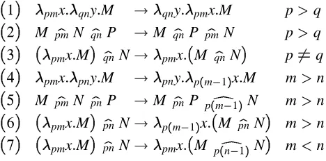
Since we have a sum, it is natural to think of a product. That is, the calculus over the set of labels which is the Cartesian product of symbolic and numeric label. Namely, a label in now a pair symbol-numeral inL =SN. This system corresponds to a calculus of named channels on which only numeric positions are considered. Per channel name, relative numeric position arguments can be done in that relative reordering of distinct positions is allowed. In a sense, it is orthogonal to the sum system, in that it separates names and numbers, although it provides each with the functionality of label-selective-reduction.
-Reduction for product, as for the sum, requires identically labeled abstractor and applicator:
() (pmx:M) b
pmN![N=x]M
As for reordering, we need only slightly alter reordering rules of the sum system as shown in Figure 2. Clearly, all proofs done above on selective-calculus are still valid for this system: we take care of numbers only when symbols are identical, and have then the same rules.
4.2 Polynomial systems
If we have sums and products, we should be able to combine them. A polynomial system is defined by two mutually exclusive sets of namesSandT, and taking the set of labels to be L=S[ T N
(1) pmx:qny:M !qny:pmx:M p>q (2) M
b
pmN qnb P
!M b
qnP pmb N p
>q (3) (pmx:M)
b
qn N!pmx:(M
b
qnN) p6=q
(4) pmx:pny:M !pny:p (m 1)x
:M m>n (5) M
b
pmN pnb P
!M b
pnP pd
(m 1)N m >n (6) (pmx:M)
b
pn N!p
(m 1)x :(M
b
pnN) m>n
(7) (pmx:M) b
pn N!pmx:(M
d
p(n 1)N
[image:31.612.167.401.90.206.2]) m<n
Figure 2: Reordering rules for polynomial system
M::=xjpx:Mjqnx:MjM bpM
0 jM
b
qnM
0
with p inSand q inT.
We just take Rules(1)–(3)of selective-calculus applied onS[ T N
and Rules (4)–(7)of product systems, applied onT.
Selective-calculus is a polynomial system whereT is restricted to an unique constructor , abbreviated.
It is only for clarity that proofs where given for selective-calculus, rather than for any polynomial system, where they are anyway valid. We should always keep in mind that when we prove or build something on selective-calculus it will be nearly always generalizable to any polynomial system, for which we are just using an abbreviated notation.
5 Towards a transformation calculus
We will just give here a new notation, and explain in what way this notation suggests another extension of selective-calculus.
The intuition behind selective -calculus is no longer functions but functions over labeled arguments which behave like communicating processes through named or (relatively) numbered channels. Application corresponds to process communication. What we called entities are seen as actions: abstractors correspond to receiving and applicators to sending. But what about composition? It is easily defined for functions as fg=f:g:x:f(gx)in the classical calculus. We could of course think of a labeled composition one for each label. But this is rather weak. Particularly when we think of the powerful out-of-order currying power of our system.
Rather, we will just change notations, and define:
M_
p x
def =px:M
at once. Here again P is a sequence of actions, and we would like to manipulate them as such. The potential of this notation is such that it simplifies considerably many proofs. For instance we could prove easily B¨ohm’s expansion theorem using it. Since our extension is conservative, our proof is valid for classical-calculus as well.
Of course, all this starts to be strongly reminiscent of a calculus for process communica-tion [12], although still a direct and conservative extension of classical-calculus. We believe that this is not coincidental. This idea is the object of our current research and we are actively exploring the deep connections with the various existing communication calculi. But, we shall say no more on this for now.
6 Conclusion and further work
Label-selective -calculus offers the advantage of realizing directly a more complete isomorphism of Cartesian products and function applications. An immediate consequence is a more convenient notation, and a more efficient, indeed concurrent, manner to extract arguments out of order.
Beyond the bare calculus, we have started studying a typed version of our calculus [6]. There, we propose a simply typed version of this calculus, and show that it extends to second order and polymorphic typing. For this last one there exists a most generic type, and we give the algorithm to find it.
A topic for further work along this idea is, of course compilation. As mentioned in the first section, we plan to extend the stack-based model of execution of-calculus with our label-selection scheme to realize efficient access to arguments regardless of position label. We have already adapted the calculus of explicit substitutions [1], as are currently working on a compiling scheme for label-selective-calculus based on it.
Also, we plan to study the work of Ohori [13] to elucidate the gains that this may have in the compilation of records. As for semantics, we have initiated work on a typed version of label-selective-calculus and a framework of models for it.
We have formulated and are studying several concurrent calculi extending label-selective -calculus towards full concurrency [2], including the provision for computable channel names. One of the gains expected is that-calculus will need not be encoded as in [11], but directly embedded as syntactic identity.