SRC RR 84A pdf

84

Graphical Fisheye Views of Graphs

Manojit Sarkar and Marc H. Brown

Systems Research Center

DEC’s business and technology objectives require a strong research program. The Systems Research Center (SRC) and three other research laboratories are committed to filling that need.

SRC began recruiting its first research scientists in l984—their charter, to advance the state of knowledge in all aspects of computer systems research. Our current work includes exploring high-performance personal computing, distributed com-puting, programming environments, system modelling techniques, specification technology, and tightly-coupled multiprocessors.

Our approach to both hardware and software research is to create and use real systems so that we can investigate their properties fully. Complex systems cannot be evaluated solely in the abstract. Based on this belief, our strategy is to demon-strate the technical and practical feasibility of our ideas by building prototypes and using them as daily tools. The experience we gain is useful in the short term in enabling us to refine our designs, and invaluable in the long term in helping us to advance the state of knowledge about those systems. Most of the major advances in information systems have come through this strategy, including time-sharing, the ArpaNet, and distributed personal computing.

SRC also performs work of a more mathematical flavor which complements our systems research. Some of this work is in established fields of theoretical computer science, such as the analysis of algorithms, computational geometry, and logics of programming. The rest of this work explores new ground motivated by problems that arise in our systems research.

DEC has a strong commitment to communicating the results and experience gained through pursuing these activities. The Company values the improved understand-ing that comes with exposunderstand-ing and testunderstand-ing our ideas within the research community. SRC will therefore report results in conferences, in professional journals, and in our research report series. We will seek users for our prototype systems among those with whom we have common research interests, and we will encourage collaboration with university researchers.

Graphical Fisheye Views of Graphs

Manojit Sarkar and Marc H. Brown

Publication History

A preliminary version of this report will appear in the Proceedings of the ACM

SIGCHI ’92 Conference on Human Factors in Computing Systems, May 1992.

Author Affiliation

Manojit Sarkar is currently a Ph.D. candidate at Brown University. The bulk of the work described here was performed while he was supported by a research internship from SRC during the summer of 1991. Subsequent work has been supported in part by ONR Contract N00014–91–J–4052, ARPA Order 8225.

Copyright and Reprint Permissions

c

Digital Equipment Corporation 1992

Abstract

Contents

1 Introduction 1

2 Terminology 3

3 A Formal Model 6

4 An Implementation Strategy 7

4.1 Computing Position : : : : : : : : : : : : : : : : : : : : : : : : 7 4.2 Computing Size : : : : : : : : : : : : : : : : : : : : : : : : : : 10 4.3 Computing Detail : : : : : : : : : : : : : : : : : : : : : : : : : 10 4.4 Computing Visual Worth : : : : : : : : : : : : : : : : : : : : : : 11 4.5 Mapping Edges : : : : : : : : : : : : : : : : : : : : : : : : : : 11

5 Another Implementation Strategy 12

6 The Prototype System 15

6.1 Implementation : : : : : : : : : : : : : : : : : : : : : : : : : : 16 6.2 Response Time : : : : : : : : : : : : : : : : : : : : : : : : : : : 17 6.3 System Notes : : : : : : : : : : : : : : : : : : : : : : : : : : : 17

7 Generalized Fisheye Views 18

8 Related Work 19

9 Summary 22

Acknowledgments 22

References 23

List of Figures

1

Introduction

Graphs with hundreds of vertices and edges are common in many areas of computer science, such as network topology, VLSI circuits, and graph theory. There are literally hundreds of algorithms for positioning nodes to produce an aesthetic and informative display [1]. However, once a layout is chosen, what is an effective way to view and browse the graph on a workstation?

Displaying all the information associated with the vertices and edges (assuming it can even fit on a screen) shows the global structure of the graph, but has the drawback that details are typically too small to be seen. Alternatively, zooming into a part of the graph and panning to other parts does show local details but loses the overall structure of the graph. Researchers have found that browsing a large layout by scrolling and arc traversing tends to obscure the global structure of the graph [6]. Using two or more views — one view of the entire graph and the other of a zoomed portion — has the advantage of seeing both local detail and overall structure, but has the drawbacks of requiring extra screen space and of forcing the viewer to mentally integrate the views. The multiple view approach also has the drawback that parts of the graph adjacent to the enlarged area are not visible at all in the enlarged view(s).

This paper explores a fisheye lens approach to viewing and browsing graphs. A fisheye view of a graph shows an area of interest quite large and with detail, and shows the remainder of the graph successively smaller and in less detail. Thus, a fisheye lens seems to have all the advantages of the other approaches without suffering from any of the drawbacks.

A typical graph is displayed in Figure 1, and fisheye versions of it appear in Figures 2–6. In the fisheye view, the vertex with the thick border is the current point of interest to the viewer. We call this point the focus. In our prototype system, a viewer selects the focus by clicking with a mouse. As the mouse is dragged, the focus changes and the display updates in real time. The size and detail of a vertex in the fisheye view depend on the distance of the vertex from the focus, a preassigned importance associated with the vertex, and the values of some user-controlled parameters. All figures in this paper are screen dumps of views generated by our prototype system.

[image:9.612.151.460.148.352.2]

Figure 1: A graph with 134 vertices and 338 edges. The vertices represent major cities in the United States, and the edges represent paths between neighboring cities. (Typically, the edges would be annotated with the distance and driving time between the cities.) The

a priori importance value assigned to each vertex is proportional to the population of the

corresponding city. Fisheye views of this graph appear in Figures 2–6

from the focus and the object’s preassigned importance in the global structure. In Furnas’s original formulation of the fisheye view, a component is either present in full detail or is completely absent from the view, and there is no explicit control over the graphical layout.

The next section defines the terminology and conventions used in the remainder of this paper. In Section 3 we present a formal model for generating graphical fisheye views. Section 4 describes the strategy we used to implement the formal model, and Section 5 describes a second implementation strategy that we explored. Section 6 describes our prototype system. In Section 7, we describe generalized fisheye views (of the sort that Furnas described), and show how an implementation of our formal model can be used for creating generalized fisheye views. In the remaining sections, we review related efforts, and offer some thoughts on future directions.

[image:10.612.155.463.134.352.2]

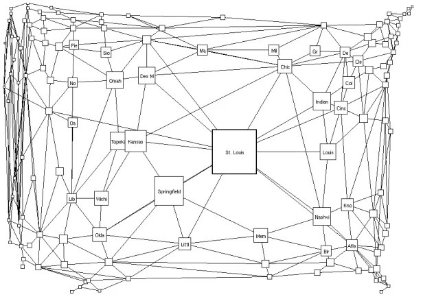
Figure 2: A fisheye view of the graph in Figure 1. The focus is on St. Louis. (The values of the fisheye parameters ared=5;c=0;e=0;VWcutoff =0; the meanings of these

parameters are explained in Sections 4 and 6.)

2

Terminology

A graph consists of vertices and edges. The initial layout of the graph is called the normal view of the graph, and its coordinates are called normal coordinates. Vertices are graphically represented by shapes whose bounding boxes are square (chosen arbitrarily). Each vertex has a position, specified by its normal coordinates, and a size which is the length of a side of the bounding box of the vertex. Each vertex is also assigned a number to represent its relative importance in the global structure. This number is called the a priori importance, or the API, of the vertex. An edge is represented by either a straight line from one vertex to another, or by a set of straight line segments to simulate curved edges. An edge consisting of multiple straight line segments is specified by a set of intermediate bend points, the extreme points being the coordinates of its corresponding vertices.

The coordinates of the graph in the fisheye view are called the fisheye

coordi-nates. The viewer’s point of interest is called the focus; it is a point in the normal

[image:11.612.157.463.78.292.2]

Figure 3: A fisheye view of the graph in Figure 1, with less distortion than in Figure 2. The values of the fisheye parameters ared=2;c=0:5;e=0:5;VWcutoff =0.

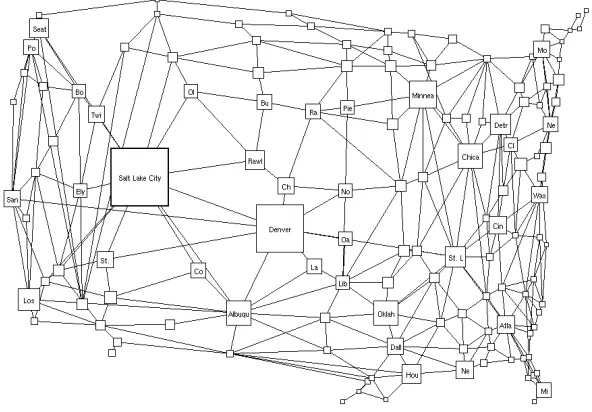
Figure 4: A fisheye view of the graph in Figure 1, with the focus on Salt Lake City. The level of distortion is the same as in Figure 3; only the location of the focus has changed. The values of the fisheye parameters ared=2;c=0:5;e=0:5;VWcutoff =0.

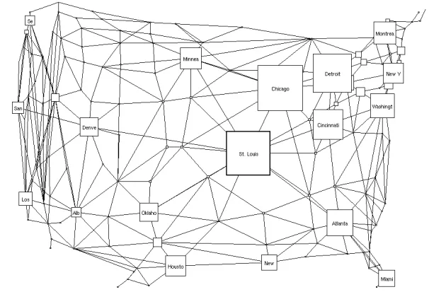
[image:11.612.158.454.368.574.2]

[image:12.612.150.465.67.282.2]

Figure 5: A fisheye view of the graph in Figure 1. Compare this to Figure 3, with the same distortion and the same focus. Here, the important vertices are larger than in Figure 3, but the unimportant ones are smaller. The values of the fisheye parameters are

d=2;c=0:75;e=0:75;VWcutoff=0.

[image:12.612.164.440.385.583.2]

amount of detail to display. Finally, each vertex in fisheye view is assigned a visual worth, or VW, computed based on its distance to the focus (in normal coordinates)

and its a priori importance.

3

A Formal Model

Generating a fisheye view involves magnifying the vertices of greater interest and correspondingly demagnifying the vertices of lower interest. In addition, the positions of all vertices and bend points must also be recomputed in order to allocate more space for the magnified portion so that the entire view still occupies the same amount of screen space.

Intuitively, the position of a vertex in the fisheye view depends on its position in the normal view and its distance from the focus. The size of a vertex in the fisheye view depends on its distance from the focus, its size in the normal view, and its API. The amount of detail displayed in a vertex in turn depends on its size in the fisheye view. We now formalize these concepts.

The position of vertex v in the fisheye view is a function of its position in normal coordinates and the position of the focusf:

P

feye

(v;f)=F1(P

norm

(v);P

norm

(f)) (1) The size of a vertex in the fisheye view is a function of its size and position in normal coordinates, the position of the focus, and its API:

S

feye

(v;f)=F2(S

norm

(v);P

norm

(v);P

norm

(f);API(v)) (2) The amount of detail to be shown for a vertex depends on the vertex’s size in the fisheye view and the maximum detail that can be displayed:

D TL

feye

(v;f)=F3(S

feye

(v;f);D TL

max

(v)) (3) Finally, the visual worth of a vertex depends on the distance between the vertex and the focus in normal coordinates (found by examining the positions of the vertex and the focus in normal coordinates) and on the vertex’s API:

VW(v;f)=F4(P

norm

(v);P

norm

(f);API(v)) (4) One has to choose the functionsF1,F2,F3,F4appropriately to generate useful fisheye views. Readers familiar with Furnas’s work will note that our fundamental contributions are the existence of arbitrary functionsF1,F2, andF3. In the next section, we present the set of functions we used in our prototype system.

[image:14.612.221.394.139.314.2]

Figure 7: An undistorted nearly-symmetric graph. This graph will be a useful basis for understanding the fisheye transformations in Sections 4 and 5.

4

An Implementation Strategy

Generating fisheye views is a two step process. First we apply a geometric trans-formation to the normal view in order to reposition vertices and magnify and demagnify areas close to and far away from the focus respectively. Second, we use the API of vertices to obtain their final size, detail, and visual worth.

4.1

Computing Position

Transforming a pointP

norm

from normal coordinates to fisheye coordinates, using focus positionP

focus

, requires us to implement the functionF1in Equation 1. We map thexandycoordinates independently as follows:

P

feye

= D

G

D

norm

x D

max

x

D

max

x +P

focus

x;

G

D

norm

y D

max

y

!

D

max

y+P

focus

y E

(5)

where

G(x)=

(d+1)x dx+1

Here,D

max

x is the horizontal distance between the boundary of the screen and the focus in normal coordinates, andD

norm

x is the horizontal distance between the point being transformed and the focus, also in normal coordinates. We divide

D

norm

x by D

max

x so that the argument toGis normalized to be between 0 and 1. Multiplying the results of G byD

max

x unnormalizes the “fisheye distance,” so that adding the position of the focus (which is the same in normal and fisheye coordinates) yields the fisheye coordinates. The meanings ofD

max

y andD

norm

y are similar, in the vertical dimension.

The constantdin functionGis called the distortion factor. The functionG(x) is monotonically increasing and continuous for 0 x 1 withG(0) = 0, and

G(1)=1. The derivative ofG(x)is

G 0

(x)=

d+1 (dx+1)

2 (7)

This indicates that for large values of d the slope of the plot of x versusG(x)near

x=0 is very large. This results in high magnification. The plot has a very small slope nearx=1 which causes high demagnification. A graph ofG(x)ford=0 andd=5 is as follows:

G(x) G(x)

x x

d = 0 _{d = 5}

0 0 0 1 0 1 1 1 magnification demagnification

Whend=0, the normal and the fisheye coordinates of every point are the same. In our prototype system, the user can interactively modify the value ofd. The effect of alteringdon the fisheye view can be seen by comparing Figure 2 to Figure 3, and Figure 7 to the columns of images in Figure 8.

We call the mapping in Equation 6 the cartesian transformation. Later, we show a slightly different transformation called the polar transformation.

[image:16.612.142.473.63.567.2]

Figure 8: Fisheye views of the nearly-symmetric graph from Figure 7 using a cartesian mapping. The left column uses a focus in the northwest, and the right column uses a focus in the southeast. The distortion increases from top to bottom: In the top rowd=1:46, in

the middle rowd=2:92, and in the bottom rowd=4:38. Note that the thickness of each

4.2

Computing Size

While computing size, the square shape of the bounding boxes of the vertices is preserved. The size mapping functionF2 in Equation 2 is implemented in two steps. The first step uses the geometric transformation just found in order to compute the geometric size S

geom

(v;f) by ignoringv’s API. This mapping has the special property that if no two vertices in the normal view overlapped, no two vertices in the transformed view overlap. The second step then usesS

geom

(v;f) andv’s API to complete the implementation ofF2. However, the vertices may overlap after the second step.

The geometric size of a vertex is found by comparing the fisheye coordinates of the vertex with a point that is on the perimeter of the vertex’s bounding box. To be precise, let’s call the length of a side of the bounds box of the undistorted vertex

S

norm

, and introduce another parameters, called the vertex-size scale factor, that the user will be able to control in our prototype system. We take a point that is

sS

norm

=2 away from the center of the vertex in the direction away from the focus, and transform it toQ

feye

usingF1in Equation 5. (Because magnification decreases as we move away from the focus, taking a point farther away from the focus rather than closer to the focus is conservative. It ensures that vertices that do not overlap in the normal view do not overlap in the fisheye view either.)

Now, the geometric size is simply

S

geom

=2 min(

Q

feye

x P

feye

x ; Q

feye

y P

feye

y

):

The minimum function keeps the bounding box square. The factor of 2 converts back into the length of a side.

Finally, the functionF2in Equation 2 is implemented by

S

feye

=S

geom

(cAPI)

e

(8) where the coefficientcand exponenteare constants. In our prototype system, the user can interactively control the values ofc,e, and alsos. Figures 3 and 5 show the effects of varying these parameters.

4.3

Computing Detail

We implemented functionF3as follows:

D TL

feye

(v;f)=min(D TL

max

(v);S

feye

(v;f)) (9) whereis a constant.

4.4

Computing Visual Worth

We implemented functionF4as follows:

VW(v;f)=S

feye

(v;f)+ (10)

whereandare constants.

Although our prototype system does not let the user control the values of,, and, the user can control the minimum level of visual worth that is necessary in order for a vertex to be displayed. Compare Figure 5 with Figure 6.

4.5

Mapping Edges

Straight line edges of the normal view are mapped to straight line edges in the fisheye view automatically when vertices at their end points get mapped. The edges with intermediate bend points are mapped by mapping each bend point separately. Figure 8 demonstrates the effect of cartesian transformations on a symmetric graph. Note in particular that parallelism between lines is not preserved, except for vertical and horizontal lines.

Unfortunately, mapping just the end points of edges may lead to edges that intersect in the fisheye view but not in the normal view. This artifact is quite noticeable in the border between Washington and Idaho in Figure 11. Fortunately, this problem is easily circumvented by mapping a large number of intermediate points on each straight line segment individually. Mapping many points on each edge would result in curved lines with the property that if the edges did not intersect in the normal view, the edges will not intersect in the fisheye view. However, mapping a very large a number of points may not be computationally feasible for real time response.

5

Another Implementation Strategy

Early users of our prototype system commented that transformations seemed some-what unnatural, especially when applied to familiar objects, such as maps. Our framework allows us to address this complaint by using domain-specific transfor-mations.

Consider for instance, the non-fisheye view of a map of the United States shown in Figure 9 and a corresponding fisheye view in Figure 10. A more natural fisheye view of such a map might be to distort the map onto a hemisphere, as is done in Figure 11. To do so, we developed a transformation based on the polar coordinate system with the origin at the focus. In this transformation, a point with normal coordinates(r

norm

; )is mapped to the fisheye coordinates(r

feye

; )where

r

feye

=r

max

(d+1)

r

r

norm

max

d

r

r

norm

max +1

(11)

[image:19.612.176.437.431.609.2]

Here, r

max

is the maximum possible value ofr in the same direction as . Note that remains unchanged by this mapping. Figure 12 shows the polar transformations on the nearly-symmetric graph from Figure 7. It is instructive to compare these mappings with the cartesian transformations of the same nearly-symmetric graph in Figure 8.

Figure 9: An outline of the United States

[image:20.612.185.425.140.315.2]

Figure 10: A cartesian transformation of Figure 9. The focus is at the point where Missouri, Kentucky, and Tennessee meet.

[image:20.612.190.426.373.544.2]

[image:21.612.141.475.61.572.2]

Figure 12: Fisheye views of the nearly-symmetric graph from Figure 7 using a polar mapping. As in Figure 8, the left column uses a focus in the northwest, and the right column uses a focus in the southeast. The distortion increases from top to bottom: In the top rowd = 1:46, in the middle rowd =2:92, and in the bottom row d= 4:38. The

thickness of each edge varies with the sizes of the vertices it joins.

Another factor contributing to the perceived unnaturalness of the fisheye view is that the shapes of vertices remain undistorted and edges remain straight lines (ignoring bend points). We could remedy this by mapping many points on the outline of the vertex, and mapping a large number of intermediate points for the edges, thus allowing the vertices and edges to become curved. However, in our prototype system, we chose not to do so, in order to achieve real time performance.

6

The Prototype System

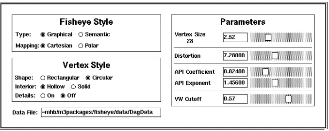
[image:22.612.138.477.476.611.2]

Our system displays a fisheye view of a user-specified graph, and updates the display in real time as the user moves the focus by dragging with the mouse. The graph is displayed in one top-level window and the control panel, shown in Figure 13, is displayed in another top-level window. The control panel has sliders and numeric typein boxes that allow the user to control of the value of the distortion factor din Equation 6, the coefficient c, exponente, and vertex scaling factors in Equation 8, and a cutoff point at which vertices and their incident edges should no longer be displayed. The coefficient c, the exponent e, and the vertex scaling factor s control the effect of the API of the vertices on the non-geometric part of the transformation, while d affects the geometric part of the transformation. The combined effect of these parameters on the graph in Figure 1 is illustrated in Figures 2– 6.

6.1

Implementation

The prototype is implemented in an event-driven style. Each time the user moves the mouse while the button is held down, the function GetFocus returns the position of the mouse:

loop

f :=GetFocus() iff 6=f

old then

foreachv V

evalP

feye

(v;f);S

feye

(v;f);D TL

feye

(v;f) endfor

foreache E

if not straightLine(e) then foreach bpbendPoints(e)

mapPoint(bp;f) endfor

endif endfor foreachv V

eval VW(v;f) endfor

foreache E

if VW(e:v1)VWcutoff and VW(e:v2)VWcutoff then

repaint edge betweene:v1ande:v2 endif

endfor

sortV in order of VW

foreachv V in nondecreasing order of VW if VW(v)VWcutoff then

repaint vertexv endif

endfor

f

old :=f endif endloop

The system normally ensures that the location of the focus is the same in both normal and fisheye coordinates. However, when the cursor is within the boundary of a vertex, the vertex becomes the focus vertex and the view is not updated until the cursor exits the vertex. Since the size of the focus vertex is usually large, exiting the focus vertex causes a relatively large shrinkage in the size of the focus vertex and also a relatively large variation in the fisheye view. In particular, since the entry and exit events happen at two different distances from the center of the focus vertex, without careful coding an exit event causes the most recent focus vertex to shift away by a large distance from the cursor in a jerky motion. One approach to solving this problem is to force the cursor to be positioned just outside the boundary of the most recent focus vertex on each exit event.

Sorting the vertices in order of their visual worth produces a very useful order. First, if the position of two vertices are in conflict, their VW can be used to resolve the conflict in favor of displaying the vertex with higher VW. Second, the order can be used to maintain the real time response of the system, as we shall discuss below.

6.2

Response Time

Our prototype system is able to maintain real time response on a DECstation 5000 for graphs of up to about 100 vertices and about 100 horizontal or vertical edges. Computing fisheye views takes an insignificant amount of time compared to the time required for painting. Real time response cannot be maintained for graphs with significantly larger number of vertices and edges. Performance also suffers when the percentage of edges that are neither horizontal nor vertical is increased.

An alternative “inner loop” is to display “approximate” fisheye views by paint-ing only a fixed number of vertices and edges, irrespective of the size of the graph. Each time there is a new focus, quickly compute the new fisheye view for all vertices, but repaint only those nodes and edges which will give the best approx-imation to the perfect fisheye view. Nodes with highest change in their VW and nodes with highest current VW are good candidates. One can take a suitable mix of these two types of nodes, as well as all the associated edges. Each update operation will then involve erasing and painting a fixed number of nodes and edges.

6.3

System Notes

small examples in the distribution package.1 A number of features that we needed for real time animation (e.g., fast double buffering), and aesthetic drawings (e.g., curved lines) were not functional when the prototype system was developed during the summer of 1991.

7

Generalized Fisheye Views

Our work follows from the generalized fisheye views by Furnas [4, 5]. Furnas gave many compelling arguments describing the advantages of fisheye views, and performed a number of experiments to validate his claims. The essence of Furnas’s formalism is the “degree of interest” function for an “object” relative to the “focal point” in some “structure.” Our notion of “visual worth” (see Equation 4) is nearly identical to Furnas’s degree of interest. The difference is that we have (thus far) described distance as the Euclidean distance separating two vertices in a graph, whereas Furnas defined the distance function as an arbitrary function between two objects in a structure. Our system supports generalized fisheye views by recoding the distance function used explicitly in Equation 4 and implicitly by Equations 1–3. For instance, consider the graph in Figure 14 and the graphical fisheye view of it in Figure 15. The distance between vertices is their Euclidean distance. A vertex is displayed only if its visual worth is above some threshold, and its position, size, and level detail are computed using Equations 1, 2, and 3, respectively. A “generalized” fisheye view of that same graph, with the same focus, is shown in Figure 16. Here, the API is as before, but the distance function not geometrical; it is the length of the shortest path between a vertex and the vertex defining the focus, as proposed by Furnas [5]. Notice that in the generalized fisheye view, each node is either displayed or omitted; there is no explicit way to vary size and level of detail.

Furnas raised the question of multiple foci [5], but left it unanswered. Our framework can be extended to multiple foci. For instance, a simplistic approach would be to divide the screen-space among all the foci using some criteria, and then apply the transformation independently on each portion of the screen.

1_{A Modula-2 version of Trestle that doesn’t use the X-toolkit has been operational for a number}

of years at DEC SRC; it has many non-trivial clients.

8

Related Work

Furnas cites a delightful 1973 doctoral thesis by William Farrand [3] as one of the earliest uses of fisheye views of information on a computer screen. The thesis suggests transformations similar to our cartesian and polar transformations, but provides few details.

At CHI ’91, Card, Mackinlay, and Robertson presented two views of structured information that have fisheye properties. The perspective wall [7] maps a wide 2-dimensional layout into a 3-dimensional visualization. The center panel shows detail, while the two side panels, receding in the distance, show the context. The cone tree [9] displays a tree with each node the apex of a cone, and the children of the node positioned around the rim of the cone. The fact that the tree is beautifully rendered in 3D, including shadows and transparency, provides the basic fisheye property of showing local information in detail (because when it is close to the synthetic camera rendering the scene it is large), while also showing the entire context (because of transparency and shadows). It would be interesting to experimentally compare cone trees and generalized graphical fisheye views as techniques for visualizing hierarchical information.

[image:27.612.175.445.238.479.2]

Figure 14: A graph with 100 vertices and 124 edges. All edges point downwards. The API of each vertex is related to its display level (e.g., the root has the highest API of 8, node 33 has an API of 4, and node 86 has an API of 2).

[image:28.612.193.420.85.274.2]

Figure 15: A graphical fisheye view of Figure 14. The focus is the vertex labeled 48.

[image:28.612.189.416.337.593.2]

9

Summary

The fisheye view is a promising technique for viewing and browsing structures. Our major contribution is to introduce layout considerations into the fisheye formalism. This includes the position of items, as well as the size and level of detail displayed, as a function of an object’s distance from the focus and the object’s preassigned importance in the global structure. A second contribution is the notion of a normal coordinate system, thereby allowing layout to be viewed as distortions of some normal structure. As we pointed out, our contributions apply to generalized fisheye views of arbitrary structures (by changing the interpretation of “distance”), in addition to graphs.

It is important to realize that we do not claim that a fisheye view is the correct way to display and explore a graph. Rather, it is one of the many ways that are possible. Discovering and quantifying the strengths and weaknesses of fisheye views are challenges for the future.

Acknowledgments

Jorge Stolfi helped with various ideas concerning geometric transformations. Steve Glassman, Bill Kalsow, Mark Manasse, Eric Muller, and Greg Nelson extricated us from numerous Modula-3 and Trestle entanglements. Mike Burrows and Lucille Glassman helped to improve the clarity of this presentation. Finally, George Furnas provided us with a wealth of information that improved many aspects of our prototype system and also of this paper.

References

[1] Peter Eades and Roberto Tamassia. Algorithms for drawing graphs: An an-notated bibliography. Technical Report CS–89–90, Department of Computer Science, Brown University, Providence, RI, 1989.

[2] Kim M. Fairchild, Steven E. Poltrok, and George W. Furnas. SemNet: Three-dimensional graphic representations of large knowledge bases. In Cognitive

Science and Its Applications for Human Computer Interaction, pages 201–

233, 1988.

[3] William Augustus Farrand. Information display in interactive design. Ph.D. Thesis, Department of Engineering, UCLA, Los Angeles, CA, 1973.

[4] George W. Furnas. The fisheye view: A new look at structured files. Technical Memorandum 82–11221–22, Bell Laboratories, 1982.

[5] George W. Furnas. Generalized fisheye views. In Proc. ACM SIGCHI ’86

Conf. on Human Factors in Computing Systems, pages 16–23, 1986.

[6] Tyson R. Henry and Scott E. Hudson. Interactive graph layout. In Proc. ACM

SIGGRAPH, SIGCHI Symposium on User Interface Software and Technology,

pages 55–65, 1991.

[7] Jock D. Mackinlay, George G. Robertson, and Stuart K. Card. The perspective wall: Detail and context smoothly integrated. In Proc. ACM SIGCHI ’91 Conf.

on Human Factors in Computing Systems, pages 173–179, April 1991.

[8] Greg Nelson, Editor. Systems Programming with Modula-3. Prentice Hall, Englewood Cliffs, NJ, 1991. Chapter 7 describes the Trestle window system.

[9] George G. Robertson, Jock D. Mackinlay, and Stuart K. Card. Cone Trees: Animated 3D visualizations of hierarchical information. In Proc. ACM

SIGCHI ’91 Conf. on Human Factors in Computing Systems, pages 189–

About the Title Page

The images on the title page are views of a graph representing the Paris Metro system. The vertices in the graph are the stations, and the edges are the routes between stations. All images are screen dumps from the prototype system described in this paper.

The upper-left image is a normal view of the Metro; the other images are fisheye views of the Metro. In all graphs, the a priori importance (API) assigned to each station is the number of connecting stations.

In the upper-right image, the sizes of vertices vary according to the API of each station. The focus is the Montparnasse-Bienvenue station, displayed as a hollow circle. The user selects a focus by clicking with the mouse.

In the lower-right image, the vertices that are close (using Euclidean distance) to the focus station are magnified, and those far away are shrunk. In addition, the locations of all vertices are changed slightly in order to give the larger vertices more space.

In the lower-left image, the focus station is changed to be Republique, and the representation of the vertices is changed to one that displays the name of the station, space permitting.

Of course, a series of static snapshots cannot not do justice to an interactive system: You need to use your imagination to visualize how the upper-right image smoothly transformed into the lower-right image, as the user moved a slider con-trolling the amount of “distortion” from 0 to 2. Visualize also how the lower-right image smoothly transformed into the lower-left image, as the user dragged the mouse from Montparnasse-Bienvenue to Republique.

Technical details (the meanings of which is explained in Section 4): In all images,

c =0:3,e =0:3, and VWcutoff = 0. In the upper images,d= 0. In the lower images,d=2. All transformations are polar.