Munich Personal RePEc Archive
Real Exchange Rate Misalignment in
Azerbaijan
Hasanov, Fakhri and Huseynov, Fariz
Institute of Cybernetics, Azerbaijan National Academy of Sciences,
North Dakota State University
2009
1
Real Exchange Rate Misalignment in Azerbaijan
Fakhri Hasanov
Senior Researcher, Institute of Cybernetics Azerbaijan National Academy of Sciences
faxri.hasanov@gmail.com
Fariz Huseynov
Assistant Professor, Department of Accounting, Finance and Information Systems College of Business, North Dakota State University, Dept 2410
PO Box 6050, Fargo, ND 58108-6050 Tel: (701) 231 5704 Fax (701) 231 6545
fariz.huseynov@ndsu.edu
2
Real Exchange Rate Misalignment in Azerbaijan
Abstract:
By using quarterly data from 2001-2007 and applying various approaches, we estimate real equilibrium exchange rate misalignment for Azerbaijani Manat (AZN) and find that AZN is slightly overvalued. Purchasing power parity approach does not explain the equilibrium exchange rate. However using behavioral and permanent equilibrium exchange rate approaches, we find that the relative productivity, terms of trade, trade openness, net foreign assets, government expenditures and oil prices are the main determinants of misalignment.
Key words: Real exchange rate, misalignment, Azerbaijan, Manat, exchange rate
JEL: F31
Introduction
Economies with inflexible nominal exchange rate regimes without necessary policies
usually face the real exchange rate misalignment. However, regardless of exchange rate
regime, monetary policy makers desire to maintain the real exchange rate close to
“equilibrium” in order to avoid negative consequences of exchange rate misalignment. Real
exchange rate misalignment is the difference between the long-run equilibrium real exchange
rate and the current real exchange rate. Consistent misalignment of the exchange rate results
in serious macroeconomic discrepancies. Several emerging, as well as, post-Soviet countries
have experienced a currency crisis because of a pegged or less flexible exchange rate regime.
Exchange rate problems and banking crises in Asia and Latin America have been studied
extensively1. In order to minimize this difference, public policy makers in transition
economies first need to estimate the key determinants of exchange rate misalignment.
The economic literature has suggested several approaches to estimate the main
determinants of misalignment. Purchasing Power Parity (PPP) approach is used as a basic
model to estimate the misalignment. However, the characteristics of transition economies may
1 Please refer to Aghion et al. (2000, 2001), Berg and Pattillo (1999a, b), Frankel and Rose (1996), Goldstein et
undermine the applicability of this approach. Several studies that employed this approach had
obtained inconsistent results. Furthermore other studies included variables, such as
productivity growth differentials, inflation rates and capital inflows to determine potential
factors influencing real exchange rates. By studying the determinants of real equilibrium
exchange rates in various transition economies, Kemme and Teng (2000), Egert and
Lahreche-Revil (2003), Kemme and Roy (2003), and Taylor and Sarno (2001) among others
find that the interest rate and productivity differentials are the key determinants of the real
exchange rate. Most of these studies use several approaches along with PPP approach, such
as Macroeconomic Balance (foreign trade balance - MB) developed by Williamson (1983,
1994), Behavioral Equilibrium Exchange Rate (BEER) suggested by Clark and McDonald
(1998, 2000), as well as Permanent Equilibrium Exchange Rate (PEER) developed by
Beveridge and Nelson (1981) to measure the misalignment in exchange rates. These methods
differ in factors they employ to estimate the misalignment. While PPP approach focus on the
nominal rate that compensate the relative price differences, MB approach use the rate that
equates domestic and foreign trade balance. However, BEER approach calculates the rate that
is determined during the long run relationship between the exchange rate and its main
determinants. The determinants can be both interest rate differentials and macroeconomic
factors. PEER approach utilizes permanent components of these variables to predict the
equilibrium real exchange rates.
To our best knowledge the previous literature has not studied the determinants of the
equilibrium real exchange rate of Azerbaijani Manat (we use Manat throughout the study) and
not identified the best approach among discussed above. Based on the findings of previous
studies, we use several methods to determine the main factors affecting the real exchange rate
in Azerbaijan. Using quarterly data from 2001-2007, we find that various PPP approaches are
caused by higher relative prices than those in main trade partners not compensated by nominal
exchange rates in the country. Macroeconomic Balance Approach also is not appropriate tool
for equilibrium exchange rate estimation, because estimated import equation (which is main
part of this approach) is not consistent with the theory. Then we apply BEER approach and
find that the main determinants of the long run REER are terms of trade index, relative
productivity, trade openness and net foreign assets. We also find a significant
Ballassa-Samuelson effect on real exchange rates with a size of 0.4 percent.
Furthermore, we find that the key determinants of the short run REER are its lagged
values, terms of trade index, trade openness, net foreign assets, and administered prices index.
The error correction approach estimates that 45 percent of misalignment in REER is restored
during one quarter. Using PEER approach we conclude that the existence of permanent
components in the long term determinants of REER increases the misalignment between
actual and equilibrium exchange rates.
The rest of the paper is designed as follows: Section I describes monetary and
exchange rate policy background for Azerbaijan. Section II estimates various PPP approaches
and makes assessments for the best approach. Section III shows the results of Macroeconomic
Balance Approach. Section IV introduces Behavioral Equilibrium Exchange Rate approach
and its results. Section V estimates Permanent Equilibrium Exchange Rate approach. Section
VI concludes.
I. Monetary and Exchange Rate Policy Background for Azerbaijan
Transition to market economy in Azerbaijan accompanied with sharp reduction in
production, hyperinflation, and depreciation of local currency. As a result, Azerbaijan
experienced volatile monetary and exchange rate policies during 90s. Eight years of war that
exacerbated these problems. However, highly volatile period was soon followed by the period
of a stable economic development in 2000s. During 2004-2007, with the implementation of
“Stability Program” supported by IMF, Azerbaijan has been able to reduce the inflationary
pressures in the economy and reach stability in prices and exchange rates. International oil
consortium linking country’s rich oil reserves with international markets through world’s
second-largest oil pipeline, BTC, created a sustainable source of rich oil revenues.
Consequently, Azerbaijan became the fastest growing country with GDP growth rate at 20-30
percent during 2005-2007. Although the oil revenues are collected in Oil Fund, the substantial
amount is transferred to government budget every year to finance infrastructure projects.
Banking industry has been country’s one of the fastest growing industries fueled by oil
revenues flown into the economy.
The developments in financial system affected foreign exchange markets in
Azerbaijan. Currently, foreign currency is traded in three trading venues: OpIFEM - Open
Interbank Foreign Exchange Market, ĐBT –Đnternal Bank Transactionns and BEST- Burse
E-System of Trade. About 40 percent of total volume is traded in IBT where firms and individual
customers exchange their currency. Total volume of transactions increased from $6.1 billion
to $15.1 billion, 50 percent of which were in dollars. Oil revenues created a large amount of
trade balance surplus that caused manat to appreciate. During 2004-2007 manat appreciated
13 percent against dollar. Appreciation in manat has increased the confidence in local
currency and manat denominated deposits grew from 20 to 50 percent of total deposits.
However, manat would further appreciate, if the Central Bank of Azerbaijan (CBA) did not
intervene to the foreign exchange markets. For example, the CBA spent $1.4 billion in 2007
(slightly less than 10 percent of total volume in dollars market) to intervene the foreign
The CBA officially states to use managed floating exchange rate regime. However,
since 1995 the fixed exchange rate regime was actually implemented with different
intermediate regimes. The CBA’s exchange rate policies varying from managed appreciation
of manat to its depreciation have been successful at attaining price and exchange rate stability.
However, increasing oil revenues forced CBA to revise its exchange rate policies and sterilize
dollar revenues. CBA’s buy-side intervention into currency markets increased inflationary
pressures. The CBA has been very flexible in its exchange rate policies recently. During 2008
the CBA pegged manat’s value to dollar, later following depreciation in dollar’s value against
euro it switched to the euro-dollar basket. Following the peak of financial crisis in October
2008, the CBA effectively dropped euro from the basket and pegged its currency to dollar.
As an oil-producing country, Azerbaijan’s macroeconomic stability is vulnerable to
right choice of exchange rate policy. Consistent misalignment in exchange rates will cause
unavoidable damages. Therefore, the aim of this study is to determine the main factors
affecting real exchange rates in Azerbaijan. Our results will provide policymakers with
effective tools to implement the right exchange rate policy.
II. PPP Approaches
A. Simplified PPP Approach
All PPP approaches suggest that the real exchange rates, R is affected from the
changes in relative price levels. These approaches estimate the real exchange rate as:
R = S * (P/P*)
where, S is nominal exchange rate, P* is the weighted average price level of trade partners
According to the relative PPP approach, we can write the nominal exchange rate as a
fraction of relation in price levels; S = k*(P*/P). Substituting this equation above we can
write: R = S * (P/P*) = k*(P*/P)* (P/P*) = k.
Simplified PPP approach assumes that the real exchange rate remains stable over the
period of time. If the rate is above the average for that period it is overvalued, otherwise the
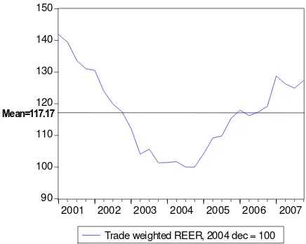
[image:8.612.191.409.226.400.2]rate is undervalued.
Figure 1: Real exchange rate time series in Azerbaijan
Figure 1 shows that the real exchange rate in Azerbaijan depreciated during 2001-2003
and appreciated since 2004. Although Central Bank of Azerbaijan (CBA) implements an
appropriate exchange rate policy to prevent Manat from appreciating, because of the increase
in oil revenues and trade balance surplus the appreciation has been inescapable since the end
of 2006. According to the Simplified APP approach real exchange rate of Manat in 2007Q4
(127.34) is 8.7 percent higher than its equilibrium level (117.18) for the given period.
However, the results should be considered with some caution, because they may be affected
by the short sample size and may differ if one considers a longer period.
B. Absolute PPP approach
90 100 110 120 130 140 150
2001 2002 2003 2004 2005 2006 2007
Another approach to test the deviations in real exchange rates is to use Absolute PPP
approach. This approach assumes that the nominal exchange rate is equal to the ratio of price
levels in domestic economy and in the main foreign trade partner:
S = P*/P or Log (S)=Log(P*) - Log(P)
We can write this equation in differences as below:
DLog(S) = DLog(P*) - DLog(P)
or
DLog(S) – (DLog(P*) - DLog(P)) = 0
Thus the change in the nominal effective exchange rates (NEER) should be equal to the
difference in home and foreign price changes. We find that the actual NEER deviates from
this definition. Figure 2 shows that changes in NEER in Azerbaijan are not equal to the
differences in home and foreign price change.
-.08 -.04 .00 .04 .08
2001 2002 2003 2004 2005 2006 2007 DLOG(NEER_T_04) DLOG(CPI_F_04)-DLOG(CPI_04)
Figure 2: NEER and differences in home and foreign prices
Alternatively, one can test the strength of Absolute PPP approach to explain the real
exchange rate misalignment by applying unit root test. This approach assumes that the
difference between home and foreign prices is offset by nominal exchange rate and the real
exchange rate remains stable or floats around that level in the long-run. This assumption will
to reject the unit root in series, then Absolute PPP approach does not hold and the real
exchange rate significantly deviates from its equilibrium.
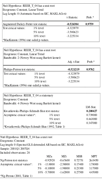
We use several methods to test for unit root in Table 1.1. The test results show that
time-series of REER is not stationary during 2001-2007, therefore we can conclude that
Absolute PPP approach cannot explain the behavior of exchange rates. In other words PPP
approach does not hold in Azerbaijani economy. However we realize that the short period of
time and the limited number of observations may affect our results and it is possible that this
approach will better fit the longer period of data.
C. PPP Adjusted for the Balassa-Samuelson and Penn Effects
In this section, we test Manat’s real exchange rate misalignment with PPP Adjusted
for the Balassa-Samuelson and Penn Effects.This approach assumes that the real exchange
rate is the change in relative prices of tradable and non-tradable goods. It can be written as:
= * * * * * T T T N T N P P P P P P S R β α
or
( )
− + + = * *
* *log *log
log log ) log( T N T N T T P P P P P P S
R
α
β
(1)where S and R are the nominal and real exchange rates, respectively, PT, PN, P*Tand P*Nare
the home and main foreign trade partner prices of tradable and non-tradable goods, while α
and β are the ratio of non-tradable goods price index to the consumer price index.
The last two terms in equation (1), the relative prices of non-tradables to tradables in
home country and in the main trade partner, estimates the Balassa-Samuelson impact. This
approach assumes that if tradables are more productive than nontradables, it will adversely
affect their prices. In other words, the prices of non-tradables will be higher than that of
tradables. This will lead to the appreciation of home currency. An increase in average
Thus if the sum of the coefficients of the third and fourth terms on the right-hand-side
of equation (1) equals to one, in other words differences in prices are offset by changing
nominal exchange rates, it is considered that the Absolute PPP approach holds true in
tradables and the real exchange rate in the country changes by relative productivity of
tradables and nontradables (or by Balassa-Samuelson effect). To test this effect, we run a
regression where the nominal effective exchange rate, relative tradables and nontradables
price index in Azerbaijan and in main trade partners are the explanatory variables. We use
CPI as a proxy for nontradables price index and PPI for tradables price index. The brief
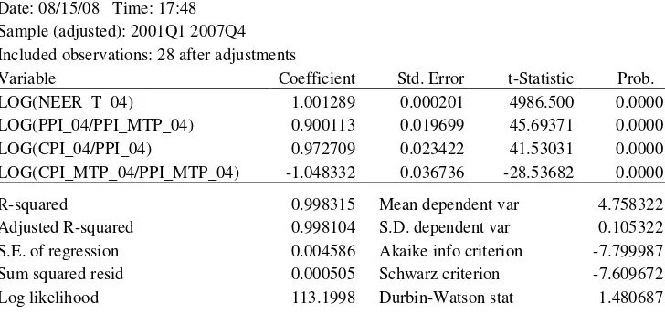
results are given below (Table 1.2):
− + + + = 4 PPI_MTP__0 CPI_MTP_04 LOG * 1.048 PPI_04 CPI_04 LOG * 0.973 PPI_MTP_04 PPI_04 LOG * 0.900 _04) LOG(NEER_T * 1.001 _04) LOG(REER_T (-28.537) (41.530) (45.694) (4986.500) : st -t (2)
where, REER is the real effective exchange rate, NEER is the nominal effective exchange rate,
PPI (CPI) producers price index (consumers price index) in home country and MTP is the
weighted average indices of main trade partners. _04 means that base year for these variables
is 2004. The numbers in brackets show the t-statistics of the coefficients.
By applying several tests, such as Durbin-Watson test, residuals test, and test for
structural breaks (test results are available upon request), we find statistically significant
results that are consistent with theoretical predictions. First, we find that there is a positive
relationship between NEER and REER. One percent increase in NEER results in one percent
increase in REER. Second, we find that tradable prices have a significant positive impact on
REER in Azerbaijan. One percent increase in tradables price index relative to the main trade
partners increases the REER by 0.9 percent. Third, the productivity, measured by the ratio of
results in 1 percent increase in REER. Finally, we also find that one percent increase in
productivity of tradables in main trade partners decrease REER by one percent.
Our findings suggest that Balassa-Samuelson effect has a significant impact on
exchange rates in Azerbaijan. This effect is determined by the relative productivity that
increases the competitiveness of goods and services produced in home country and the value
of local currency. However, one needs to be somewhat cautious while interpreting these
results. The increase in productivity observed in Azerbaijan is mostly caused by oil sector. It
is well known that the productivity in oil industry in Azerbaijan is growing while that in
non-oil sector tends to decline. However, the productivity growth in non-oil industry is mainly caused
both by increase in total output and in oil prices. Although this type of productivity does not
contribute to the competitiveness of the country and growing oil revenues cause manat to
appreciate.
An alternative way to test the Balassa-Samuelson effect is to combine the first two
variables – NEER and relative tradables price index – in the equation (1) as below:
− + = * *
* *log *log
* log ) log( T N T N T T P P P P P P S
R
α
β
This approach states that if the coefficient of the first variable is not significantly
different from zero, then REER in Azerbaijan is determined by the relative productivity in
tradables and nontradables. Our test results are given in Table 1.3. The equation is as follows:
(
)
− + + = 4 PPI_MTP__0 CPI_MTP_04 LOG * 0,968 PPI_04 CPI_04 LOG * 1,082 PPI_MTP_04 PPI_04 NEER_T_04 LOG * 1,001 _04) LOG(REER_T (-20,524) (78,802) (3515,193) : st -t * (3)We find that the coefficient of combined effect of NEER with relative tradables price
index is not insignificant. Particularly, t-statistics show that its coefficient is significantly
the firm term is not different from zero. The Wald test results (Panel B in Table 3) reject the
null hypothesis. We conclude that REER in Azerbaijan is affected not only by
Balassa-Samuelson effect, but also by NEER and the relative tradables price index.
When we compare the differences between actual and fitted values (Panel C, Table 3),
we find that the real exchange rate overvalued 0.1 percent during the last quarter of 2007 and
0.3 percent annual during 2007.
These results suggest that Absolute PPP approaches do not explain the real exchange
rate misalignment, in other words deviation in exchange rates caused by relative price
disparity is not offset by the changes in the nominal exchange rates in Azerbaijan. Indeed,
Azerbaijan has experienced higher prices than its main trade partners and this difference has
not been mitigated by manat’s depreciation which undermines the impact of Absolute PPP
approach. However, we understand that small sample size used in the study may affect our
results.
III. Macroeconomic Balance Approach
Another approach to test the misalignment in real exchange rates is Macroeconomic
Balance Approach. One of the main procedures in this approach is to estimate the import
function. The theory suggests that there is a positive relationship between a country’s imports
and the real exchange rates. In other words, the elasticity of imports to the real exchange rates
is expected to be positive. However, this is not the case for Azerbaijan. We use the real
exchange rate as an independent and real GDP as a control variable to test the impact of the
former on imports.
(
REER_T_04)
0,747*LOG(
GDP_R)
LOG * 1,339 7,154 LOG(IM_R)
(13,999) (-6,319)
(6,806) :
st -t
+ −
= (4)
The results (Table 4) are not consistent with theoretical predictions. As shown from the
currency appreciates, imports in Azerbaijan decreases. However, the economic intuition
suggests the opposite. Therefore we can conclude that Macroeconomic Balance Approach is
not appropriate to estimate REER misalignment in Azerbaijan due to the inconsistent results
of import function.
IV. Behavioral Equilibrium Exchange Rate (BEER)
Countries with higher risk will offer higher interest rates to attract capital flow which
will affect exchange rates. To account for the risk premium, BEER approach includes the
interest rates difference between countries and can be written as below:
− =
* ,
, , *), (
gdebt gdebt nfa
tnt tot r r F BEER
where r-r* is the difference between home and foreign interest rates; tot is the terms of the
trade; tnt is the productivity reflected by the ratio of tradables to non-tradables price indices
(relative of the main trade partners); nfa is the net foreign assets; gdebt/gdebt* is ratio of
domestic government debt to GDP (relative to the main trade partner)
One of the advantages of the BEER is that this approach incorporates stylized facts of
the country of interest. In this case the set of proxies for variables of interest may be affected
by country specific factors. Therefore several issues need to be considered when this approach
is applied to, particularly for Azerbaijan economy. First, net foreign assets divided by GDP
may not accurately reveal the impact of capital inflow on the real exchange rates. Because
GDP and net foreign assets are mainly consisted of oil revenues, we take the ratio of net
foreign assets to the non-oil GDP. Thus we can prevent oil factor from “contaminating” test
results. Second, interest rates will not have any significant impact on the real exchange rate
due to the lack of well-developed financial markets in Azerbaijan. Third, due to the lack of
Fourth, the strong dependence of Azerbaijani economy on oil revenues and its impact on
exchange rates require that we include oil prices variable (oil_p) into our analysis. Fifth, the
government expenditures in Azerbaijan have increasingly flown to non-oil sector. Therefore,
we adjust our approach by including the ratio of government expenditures to non-oil GDP
variable (gov_exp_ngdp) to control for this effect. Sixth, the previous studies show that it is
essential to include price index for government regulated goods to estimate BEER approach in
transition countries. We use administered prices index variable (cpi_adm) for this purposes.
Finally, previous studies also find that when using BEER approach in small and open
economies, the degree of trade openness which is calculated as the ratio of trade turnover to
GDP is essential to determine the equilibrium level of real exchange rate.
Thus, we can re-write our set of determinants of real exchange rate in BEER approach
as follows:
) , _ , _ , exp_ _ , _ , ,
(tot ntt nfa ngdp gov ngdp oil p cpi adm open
f REER =
We use the ratio of non-tradables to tradables price index for Azerbaijan and its main
trading partners (CPI/PPI)/(CPI*/PPI*) as a proxy for relative productivity (ntt). We use
quarterly data from 2001 to 2007 to test BEER approach. All variables, except oil prices,
administered CPI and government expenditures ratio to non-oil GDP, were seasonally
adjusted (_SA).
We can separate REER series in Azerbaijan into three different sub-periods:
depreciation (2001-2003), relative stability (2003-2004) and appreciation (2004-2007)
periods. We can refer to several reasons for this pattern. While the depreciation can be
explained by decreasing in the terms of trade, relative productivity and net foreign assets
position, the appreciation after 2004 may be caused by the increase in the administered prices
index, in the degree of trade openness, in relative productivity, in net foreign assets and in
BEER estimates the long-term relation or cointegration between the real exchange
rates and its macroeconomic determinants. The first step in this approach is to examine
whether the dependent variable and its determinants integrate at the same order. Desirably,
these variables must be non-stationary in level and stationary in differences. Our unit root
tests conclude that these variables are non-stationary, I(1) in level and stationary, I(0), in
differences (Table 5) at 5 percent significance level.
Because of the short sample size (28 observations) and structural breaks during last
years of sample period, we avoid using Johansen cointegration test. Instead, we use
Engle-Granger cointegration test (Engle and Engle-Granger, 1987) to estimate the BEER for Manat. Our
results (Table 6) are given below:
(
)
(
)
(
)
(
)
(
)
(
OPEN SA)
0,072*LOG(
GOV EXP NGDP)
LOG * 0,413 -ADM CPI LOG * 0,009 P OIL LOG * 0,0004 SA NGDP NFA LOG * 0,163 SA NTT LOG * 0,563 SA TOT LOG * 0,467 4,632 _04) LOG(REER_T (1,150) (-3,731) (0,103) (0,006) (2,385) (2,173) (3,107) (13,374) : st -t _ _ _ 04 _ _ _ _ _ _ _ + − + − + + + + = (5)
We find that the impact of oil prices, administered prices index and the ratio of
government expenditures to non-oil GDP on the real exchange rate are not statistically
significant. We check the robustness of our results as follows. First, by applying several tests,
such as univariate regression, Granger-Causality test, and omitted variables test, we conclude
that the relationship between administered prices index and the real exchange rates in
Azerbaijan is not statistically significant. Test results are available upon request.
Second, oil prices become insignificant in BEER approach, because of possible
interaction with other variables, such as net foreign assets and government expenditures2. In
other words, these variables can be strongly correlated with each other, because oil revenues
directly affect the net foreign assets acquisition and have a strong impact on government
2We also get statistically significant long-run and short run relationships between REER and its determinants,
revenues in Azerbaijan. Table 7 shows the correlation matrix for these variables. We find that
all three dependent variables are strongly correlated with each other, however, only net
foreign assets is somewhat strongly correlated (0.53) with REER3.
Therefore we can exclude oil prices, administered prices index and government
expenditures from equation (5). The results of revised specification are given below:
(
)
(
)
(
OPEN SA)
0,223*LOG(
NFA NGDP SA)
LOG * 0,411
SA NTT LOG * 0,423 SA TOT LOG * 0,519 4,637
_04) LOG(REER_T
(4,576) (-4,023)
(2,432) (4,472)
(139,151) :
st -t
_ _
_
_ _
+ −
− +
+ =
(6)
We find that all dependent variables included in this specification are statistically significant
and their signs are consistent with theoretical predictions. Terms of trade, relative price ratio
of nontradables to tradables, and the ratio of net foreign assets to non-oil GDP have a positive,
while trade openness has a negative impact on the real exchange rates. Our results also satisfy
several robustness tests on coefficients, residuals and the stability tests (available at reader’s
request).
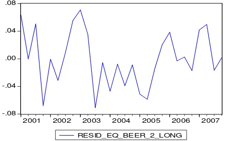
According to Engle-Granger approach (Engle and Granger, 1987) we need to test for
stationarity of residuals to conclude that there is a cointegration between REER and its
determinants. Figure 3 illustrates the time series of residuals.
Since residual series is not observable, we should not use standard critical values
(based on MacKinnon (1996)) for Augmented Dickey Fuller Unit Root Test which E-views
and other econometric packages usually perform. Therefore we use critical values of
MacKinnon (1991) table for Unit Root Test on the residuals. As shown from Table 3.14 in
Appendix 3, cointegration exists between REER and its determinants only at 90%
significance level. This is maybe because of the small sample period, since we only have 28
3 Although we do not report, Granger-Causality tests show that there is a statistically significant relation between
observations. As stated in Engle and Granger (1987), we may also use Durbin-Watson
statistics to test co-integration between variables in the Engle-Granger two-step cointegration
approach. Test results indicate existence of cointegration between REER and its
determinants4.
-.08 -.04 .00 .04 .08
2001 2002 2003 2004 2005 2006 2007
[image:18.612.190.419.175.318.2]RESID_EQ_BEER_2_LONG
Figure 3 Residuals from the BEER approach in equation (6)
We can summarize the results of BEER approach in equation (6) as follows. First, the
elasticity of REER regarding with terms of trade index is equal to 0.5 percent. This result is
consistent with the theory of the positive relationship between trade environment and home
currency. In other words, when trade environment improves, the home currency appreciates.
Second, the Balassa-Samuelson effect, indicated by the ratio of non-tradables price
index to the tradables price index, has a positive impact (0.4 percent) on REER in Azerbaijan.
In other words, rising productivity in tradables sector has led to the appreciation of home
currency. However, when this effect is closely analyzed, we find that its mostly caused by oil
sector. If we analyze oil and non-oil tradables separately, we find that non-oil sector in
Azerbaijan has not been able to increase its productivity competitiveness. Indeed, agriculture
and non-oil industrial production do not possess modern technology and high skilled human
resources in order to claim for a higher productivity. Therefore, these sectors of economy are
not able to provide foreign markets with competitive goods. On the other hand, oil production
is based on contractual agreements and not defined by the level of competitiveness.
Considering these sides of Azerbaijani economy, we can conclude that the productivity effect
defined in Balassa-Samuelson approach does not exist in Azerbaijan.
Third, we find that one percent increase in the degree of openness results in 0.4
percent depreciation in REER in Azerbaijan. This effect is common for transition economies.
Indeed, when small and open transition countries diminish foreign trade barriers, their imports
tend to rise and their home currency depreciates.
Fourth, we also find that when net foreign assets increase one percent, manat
appreciates by 0.2 percent. This result is intuitive, because higher oil prices and larger
production increase oil revenues (and net foreign assets) which leads to the appreciation of
home currency.
Based on the equation (6) we also calculate contributions of each explanatory variable
to REER during 2003-2007 (Table 10).
We can conclude that the main determinants of REER based on the BEER approach
are terms of trade, relative productivity (the ratio of non-tradables to tradables price index),
openness and net foreign asset position.
A. Short run modeling
The next step in Engle-Granger approach is to construct a short-run model between
key determinants and REER, including error correction mechanism (residuals derived from
long-run approach with one lag). The main conditions for this stage are that variables have to
be stationary in first difference, coefficient of one lagged residuals which derived from
long-run model have to be statistically significant, and its value should fall between -1 and 0. In
previous sections we concluded that the variables of interest are non-stationary in level, but
We employ a general to specific approach for the short run modeling and obtain the
specification as below:
(
)
(
)
(
)
(
)
(
CPI ADM)
0,450*RESID_EQ_B EER_2_LONG (-1) DLOG * 0,164 SA NGDP NFA DLOG * 0,075 SA OPEN DLOG * 0,232 SA TOT DLOG * 0,240 T REER DLOG * 0,237 C * 0,008 T_04) DLOG(REER_ (4,981) (3,427) (3,615) ) (-6, (3,724) (2,207) (-2,080) : st -t − + + + − + + − + = 04 _ _ _ _ _ _ ) 1 ( 04 _ _ 230 (7)Equation (7) is also robust to tests for heteroscedasticity, autocorrelation and residuals
test (Test results are available upon request). On the other hand Omitted Variables Test (Table
12) suggests that administered prices index variable should keep in the specification. The
error correction coefficient is consistent with theory; therefore we can also conclude that there
is a stable cointegration between REER and its key determinants.
Thus, short-term misalignment of REER is caused by its one period lagged values,
terms of trade, trade openness, net foreign asset position and administered prices index. The
error correction coefficient shows that misalignment from equilibrium is corrected by 45
percent during a quarter.
B. Misalignment in Real Effective Exchange Rates
We compare the actual and fitted (obtained from equation (6)) values of REER during
Figure 4. Actual (blue line) and Fitted values of REER from Engle Granger approach (red line)
We find that predicted values based on equation (6) and values of REER are very close
each other at the end of period, 4th quarter of 2007. As shown in Table 13, REER is slightly
overvalued by about 0.2 percent at the fourth quarter of 2007 and 1.9 percent annually base
respectively. Thus we can summarize our conclusions based on BEER approach as below:
a) Based on Engle-Granger approach we find that there is a statistically significant and
stable cointegration between real effective exchange rate and terms of trade, relative
productivity, net foreign assets position, and trade openness in Azerbaijan.
b) Administered prices index and lagged values of REER, along with all variables
mentioned above except relative productivity, have statistically significant impact on
REER in the short run.
c) One quarter correction in REER misalignment is equal to 45 percent.
d) The equilibrium value of REER is approximately equal to its actual values at the fourth
quarter of 2007.
5. Permanent Equilibrium Exchange Rate Approach
90 100 110 120 130 140 150
PEER approach studies the long-run relationship between actual exchange rates and
permanent components (S) of its determinants. We can write this model as below:
P t P t P t P t P t PEER t
gdebt
gdebt
nfa
tnt
tot
r
r
q
)
*
(
*)
(
1 2 3 30
β
β
β
β
β
α
+
−
+
+
+
+
=
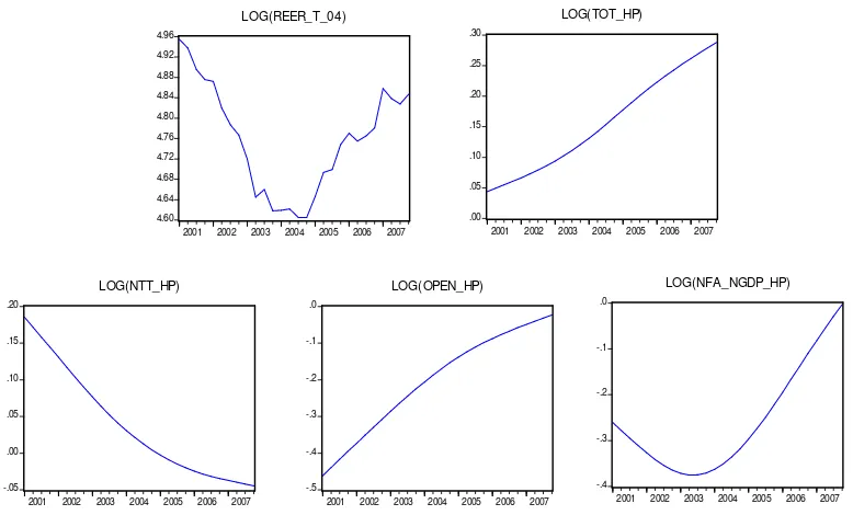
To estimate this model, first, we need to decompose permanent and transitory
components of key independent variables for what we use Hodrick-Prescott values. The
graphical illustration of REER and permanent components of key determinants over the
period 2001-2007 is given in Figure 8.
4.60 4.64 4.68 4.72 4.76 4.80 4.84 4.88 4.92 4.96
2001 2002 2003 2004 2005 2006 2007
LOG(REER_T_04) .00 .05 .10 .15 .20 .25 .30
2001 2002 2003 2004 2005 2006 2007
LOG(TOT_HP) -.05 .00 .05 .10 .15 .20
2001 2002 2003 2004 2005 2006 2007
LOG(NTT_HP) -.5 -.4 -.3 -.2 -.1 .0
2001 2002 2003 2004 2005 2006 2007
LOG(OPEN_HP) -.4 -.3 -.2 -.1 .0
2001 2002 2003 2004 2005 2006 2007
[image:22.612.103.492.280.515.2]LOG(NFA_NGDP_HP)
Figure 8. REER and permanent components of its determinants
Next, in order to estimate PEER model, we need two thing: a) the coefficients of key
determinants obtained from BEER approach (equation (6)) and b) time series of permanent
components of key determinanatsof .
(
)
(
)
(
)
(
)
+ − − + + = HP NGDP NFA LOG * 0,223 HP OPEN LOG * 0,411 HP NTT LOG * 0,423 HP TOT LOG * 0,519 4,637 EXP PEER_T_04 (4,576) (-4,023) (2,432) (4,472) (139,151) : st -t _ _ _ _ _ (8)Where, EXP is an exponential function.
Equilibrium series that derived from equation (8) and actual series of REER are illustrated in
[image:23.612.163.439.258.475.2]the Figure 9.
Figure 9. Actual (blue line) and fitted (red line) values of REER
As shown from Figure 9, the difference between blue and red lines suggest that REER
in Azerbaijan is overvalued based on PEER model. We also show actual values and
equilibrium values and the misalignments of REER based on PEER approach in Table 14.
We can conclude based on PEER approach that the size of permanent exchange rate
misalignment is about 7.3 percent in the fourth quarter of 2007, and 4.3 percent annually.
90 100 110 120 130 140 150
2001 2002 2003 2004 2005 2006 2007
Conclusion
We investigate the determinants of equilibrium level of Azerbaijani manat’s real
effective exchange rate and its misalignment in this paper. Our results can be summarized as
below:
a) The Macroeconomic Balance Approach is not relevant to estimate REER
equilibrium, due to fact thatimport function is not consistent with the theory, such
that there is a negative relation between imports and manat’s value.
b) After estimating various PPP approaches, we conclude that this group of
approaches is not appropriate for estimating equilibrium exchange rates in
Azerbaijan. In other words, deviations caused by relative prices are not completely
compensated by nominal exchange rates. This may be a result of higher relative
prices not compensated by nominal exchange rates in the country than those in
main trade partners. Alternatively, this may be caused by the short sample size.
c) Using other approaches we find that Manat is close to its equilibrium level, or
slightly overvalued such that;
d) Because of structural breaks in REER time series, we can separate it into three
subsamples – 2001-2003 when rates are depreciating, 2003-2004 when rates are
flat, and the period after 2004 when rates are appreciating. The behavior of
exchange rates during the last two sub-periods can be explained by terms of trade ,
relative productivity, net foreign assets position increased by oil revenues,
administered prices index, and by increase in government expenditures.
e) The main determinants of REER in the long run are terms of trade, relative
productivity, trade openness and net foreign assets position;
b. The size of Ballassa-Samuelson effect measured by the ratio of
nontradables to tradables price index is about 0.4 percent. In other words,
the test results suggest that productivity increase in tradables sector caused
appreciation in manat. However, one can easily realize that this is caused
by recent developments and increase in productivity, mainly, in Azerbaijani
oil industry.
c. One percent increase in trade openness lowers REER in Azerbaijan by 0.4
percent. This is consistent with the notion that when small and open
transitional countries lower foreign trade barriers, they tend to import more
and their home currency depreciates.
d. One percent increase in net foreign assets results in 0.2 percent
appreciation in Manat’s value. This result is straightforward, because along
with rising oil prices and total output, oil revenues (and net foreign assets)
of Azerbaijan increase. Thus, increasing oil revenues lead to the
appreciation of home currency.
f) The key determinants of REER in the short run are its lagged values, terms of trade
, trade openness, net foreign assets position, and administered prices index. The
error correction coefficient indicates that 45 percent of deviation of REER from its
equilibrium level is restored during one quarter.
g) We find that permanent misalignment (based on PEER approach) of REER is
bigger than its current misalignment (based on BEER approach). The impact of
permanent components increase misalignment between actual (prevailing) and
equilibrium REER in long run.
h) Finally, we provide the results of various approaches for misalignment applied in
References:
Aghion, P., Bacchetta P., Banerjee A., 2000. A simple approach of monetary policy and
currency crisis. European Economic Review 44(4-6), 728-738.
____, ____, ____ , 2001. 45(7), 1121-1150.
Berg, A., Pattillo, C., 1999a. Predicting currency crisis: the indicators approach and an
alternative. Journal of International Money and Finance 18(4), 561-86.
Berg, A., Pattilo, C., 1999b. What caused the Asian crisis: an early warning system approach.
Economic Notes 28(3), 285-334.
Beveridge, S., and Nelson C., 1981. A new approach to decomposition of economic time
series into permanent and transitory components with particular attention to
measurement of the business cycle. Journal of Monetary Economics 7, 151-74.
Clark, P.B. and MacDonald, R. (1998), “Exchange Rates and Economic Fundamentals: “A
Methodological Comparison of BEERs and FEERs” IMF Working Paper No.
WP/98/67.
Clark, P.B. and MacDonald, R. (2000), “Filtering the BEER: A Permanent and Transitory
Decomposition”, IMF Working Paper No. 00/144.
Egert, B., Lahreche-Revil, A., 2003. Estimating the fundamental equilibrium exchange rate of
central and eastern European contries: the EMU enlargement perspective. CEPII
Research Center Working Paper 2003-2005, CEPII, Paris.
Elbadawi, I. A., 1994. Estimating Long Run Equilibrium Real Exchange Rates. In:
Williamson, J. (Ed.). Estimating Equilibrium Exchange Rates. Institute for
International Economics, Washington, DC., pp. 93-131.
Engle R.F. and Granger C.W.J. "Co-Integration and Error Correction: Representation,
Estimation, and Testing", Econometrica,Vol.55,No.2. (Mar.,1987), pp. 251-276.
Frankel, J. A., Rose, A. K., 1996. Currency crashes in emerging markets: an empirical
treatment. Journal of International Economics 41(3-4), 351-66.
Goldstein, M., Kaminsky, G. L., Reinhart, C. M., 2000. Assessing Financial Vulnerability: An
Early Warning System for Emerging Markets. Institute for International Economics:
Washington, DC.
Johansen, S. (1995) Likelihood-based inference in cointegrated vector auto-regressive
Johansen, S., 1988. Statistical analysis of cointegration vectors. Journal of Economic Dynamics
and Control 12, 231-254.
Johansen, S. (2002). “A small sample correction for the test of co-integrating rank in the
vector autoregressive model”. Econometrica 70, 1929-1961.
Johansen, S., Juselius, K., 1990. Maximum likelihood estimation and inference on
cointegration with applications to the demand for money. Oxford Bulletin of
Economics and Statistics 52, 169-210.
Juselius, K., 2006. The cointegrated VAR model: methodology and applications, Oxford
University Press Inc., New York.
Kemme D. M., Roy, S., 2003. Exchange Rate Misalignment: Macroeconomic Fundamentals
as an Indicator of Exchange Rate Crisis in Transition Economies. In: Hubert, G. (Ed.).
Empirical Methods for Analyzing the Risks of Financial Crises. Institute for Economic
Research-Halle, Halle(Saale), Germany, pp. 7-32.
Kemme, D. M., Teng, W., 2000. Determinants of the real exchange rate, misalignments and
implications for growth in Poland. Economic Systems 24(2), 171-205.
Krugman, P. (Eds.), 2000. Currency Crises. The National Bureau of Economics Research,
USA. The University of Chicago Press, Chicago and London.
Liargovas, P., 1999. An assessment of real exchange rate movements in the transition
economies of central and Eastern Europe. Post-Communist Economies 11(3),
299-318.
Obstfeld, M., 1996, Approaches of Currency Crises with self-fulfilling features, European
Economic Review, 40, pp. 1037-1048.
Peter Isard, (2007) Equilibrium Exchange Rates: Assessment Methodologies, IMF Institute
IMF Working Paper December
Reza Y. Siregar and Ramkishen S. Rajan, (2006), Models of Equilibrium Real Exchange
Rates Revisited: A Selective Review of the Literature, Centre for International
Economic Studies, Discussion Paper No. 0604, August
Taylor, M. P., Sarno, L., 2001. Real exchange rate dynamics in transition economies: a
nonlinear analysis. Studies in Nonlinear Dynamics and Econometrics 5(3), 153-177.
Williamson (1983) …
Williamson, J., 1994. Estimates of FEERs. In: Williamson J. (Ed.). Estimating Equilibrium
Table 1. Unit root test results for REER during 2001-2007 This table shows various test result for unit root in REER.
Null Hypothesis: REER_T_04 has a unit root Exogenous: Constant, Linear Trend
Lag Length: 0 (Automatic based on SIC, MAXLAG=6)
t-Statistic Prob.*
Augmented Dickey-Fuller test statistic -0.526384 0.9759
Test critical values: 1% level -4.323979
5% level -3.580623
10% level -3.225334
*MacKinnon (1996) one-sided p-values.
Null Hypothesis: REER_T_04 has a unit root Exogenous: Constant, Linear Trend
Bandwidth: 2 (Newey-West using Bartlett kernel)
Adj. t-Stat Prob.*
Phillips-Perron test statistic -0.521219 0.9762
Test critical values: 1% level -4.323979
5% level -3.580623
10% level -3.225334
*MacKinnon (1996) one-sided p-values.
Null Hypothesis: REER_T_04 is stationary Exogenous: Constant
Bandwidth: 4 (Newey-West using Bartlett kernel)
LM-Stat. Kwiatkowski-Phillips-Schmidt-Shin test statistic 0.200427
Asymptotic critical values*: 1% level 0.739000
5% level 0.463000
10% level 0.347000
*Kwiatkowski-Phillips-Schmidt-Shin (1992, Table 1)
Null Hypothesis: REER_T_04 has a unit root Exogenous: Constant
Lag length: 0 (Spectral GLS-detrended AR based on SIC, MAXLAG=6) Sample: 2001Q1 2007Q4
Included observations: 28
Table 2 Absolute PPP approach with Balassa Samuelson and Penn effect
This table presents results of test for Balassa Samuelson and Penn effect in real exchange rates. REER is the real effective exchange rate, NEER is the nominal effective exchange rate, PPI (CPI) producers price index
(consumers price index) in home country and MTP is the weighted average indices of main trade partners. _04
means that base year for these variables is 2004.
Dependent Variable: LOG(REER_T_04) Method: Least Squares
Date: 08/15/08 Time: 17:48 Sample (adjusted): 2001Q1 2007Q4 Included observations: 28 after adjustments
Variable Coefficient Std. Error t-Statistic Prob.
LOG(NEER_T_04) 1.001289 0.000201 4986.500 0.0000
LOG(PPI_04/PPI_MTP_04) 0.900113 0.019699 45.69371 0.0000
LOG(CPI_04/PPI_04) 0.972709 0.023422 41.53031 0.0000
LOG(CPI_MTP_04/PPI_MTP_04) -1.048332 0.036736 -28.53682 0.0000
R-squared 0.998315 Mean dependent var 4.758322
[image:29.612.94.458.160.332.2]Adjusted R-squared 0.998104 S.D. dependent var 0.105322 S.E. of regression 0.004586 Akaike info criterion -7.799987 Sum squared resid 0.000505 Schwarz criterion -7.609672 Log likelihood 113.1998 Durbin-Watson stat 1.480687
Table 3 Absolute PPP approach with Balassa Samuelson and Penn effect
Panel A
Dependent Variable: LOG(REER_T_04) Method: Least Squares
Sample (adjusted): 2001Q1 2007Q4 Included observations: 28 after adjustments
Variable Coefficient Std. Error t-Statistic Prob.
LOG((NEER_T_04)*(PPI_04/PPI_MTP_04)) 1.001254 0.000285 3515.193 0.0000 LOG(CPI_04/PPI_04) 1.082228 0.013734 78.80155 0.0000 LOG(CPI_MTP_04/PPI_MTP_04) -0.967843 0.047156 -20.52416 0.0000
R-squared 0.996463 Mean dependent var 4.758322
Adjusted R-squared 0.996180 S.D. dependent var 0.105322
S.E. of regression 0.006509 Akaike info criterion -7.130187
Sum squared resid 0.001059 Schwarz criterion -6.987451
Log likelihood 102.8226 Durbin-Watson stat 1.183969
Panel B
Wald test results for REER approach in equation (3)
Test Statistic Value df Probability
F-statistic 12356578 (1, 25) 0.0000
Chi-square 12356578 1 0.0000
Null Hypothesis Summary:
Normalized Restriction (= 0) Value Std. Err.
C(1) 1.001254 0.000285
Panel C. Actual and fitted values of REER
Period Actual REER, 2004m12=100
Fitted REER, 2004m12=100
Misalignment, % change
2006Q4 119,185 119,454
2007Q1 128,777 128,216
2007Q2 126,259 126,335
2007Q3 124,940 125,291
2007Q4 127.338 127.261 0.060
[image:30.612.99.450.87.194.2]Annual 106.841 106.536 0.287
Table 4: Import as a Function of REER
This table shows the relation between imports and REER. IM is the amount of imports, GDP is the amount of GDP for a given period. All values are in logged terms.
Dependent Variable: LOG(IM_R) Method: Least Squares
Date: 08/16/08 Time: 17:19 Sample: 2001Q1 2007Q4 Included observations: 28
Variable Coefficient Std. Error t-Statistic Prob.
C 7.153921 1.051154 6.805781 0.0000
LOG(REER_T) -1.338630 0.211844 -6.318943 0.0000
LOG(GDP_R) 0.747009 0.053362 13.99897 0.0000
Table 5. Unit Root Test for Determinants of BEER
Group unit root test: Summary Date: 09/23/08 Time: 12:25 Sample: 2001Q1 2007Q4
Exogenous variables: Individual effects, individual linear trends Automatic selection of maximum lags
Automatic selection of lags based on SIC: 0 to 5 Newey-West bandwidth selection using Bartlett kernel
Cross-
Method Statistic Prob.** sections Obs Null: Unit root (assumes common unit root process)
Levin, Lin & Chu t* -0.35764 0.3603 8 215 Breitung t-stat 1.34201 0.9102 8 207
Null: Unit root (assumes individual unit root process)
Im, Pesaran and Shin W-stat 1.00426 0.8424 8 215 ADF - Fisher Chi-square 11.6990 0.7644 8 215 PP - Fisher Chi-square 21.6882 0.1535 8 220
Null: No unit root (assumes common unit root process)
Hadri Z-stat 6.43549 0.0000 8 224
** Probabilities for Fisher tests are computed using an asymptotic Chi-square distribution. All other tests assume asymptotic normality
Table 6. Long-run BEER approach
Dependent Variable: LOG(REER_T_04) Method: Least Squares
Date: 09/23/08 Time: 12:03 Sample: 2001Q1 2007Q4 Included observations: 28
Variable Coefficient Std. Error t-Statistic Prob.
C 4.631767 0.346337 13.37358 0.0000 LOG(TOT_SA) 0.466657 0.150189 3.107140 0.0056 LOG(NTT_SA) 0.562624 0.258912 2.173028 0.0420 LOG(OPEN_SA) -0.413067 0.110723 -3.730617 0.0013 LOG(NFA_NGDP_SA) 0.163397 0.068510 2.385015 0.0271
LOG(OIL_P) -0.000429 0.074993 -0.005714 0.9955
LOG(CPI_ADM_04) 0.009406 0.090906 0.103475 0.9186
LOG(GOV_EXP_NGDP) 0.072428 0.062979 1.150045 0.2637
[image:31.612.91.439.465.718.2]Table 7. Correlation matrix of REER, oil prices, net foreign assets and the ratio of government debt to non-oil GDP
LOG(REER_T_04) LOG(NFA_NGDP_SA) LOG(OIL_P) LOG(GOV_EXP_NGDP) LOG(REER_T_04) 1.000000 0.534172 -0.088907 0.053047
LOG(OIL_P) -0.088907 0.551969 1.000000 0.801295 LOG(NFA_NGDP_SA) 0.534172 1.000000 0.551969 0.606413
[image:32.612.83.539.111.500.2]LOG(GOV_EXP_NGDP) 0.053047 0.606413 0.801295 1.000000
Table 8. Long-run BEER approach
Dependent Variable: LOG(REER_T_04) Method: Least Squares
Date: 09/23/08 Time: 13:28 Sample: 2001Q1 2007Q4 Included observations: 28
Variable Coefficient Std. Error t-Statistic Prob.
C 4.637482 0.033327 139.1513 0.0000 LOG(TOT_SA) 0.518627 0.115966 4.472242 0.0002 LOG(NTT_SA) 0.422541 0.173712 2.432425 0.0232 LOG(OPEN_SA) -0.411059 0.102184 -4.022734 0.0005 LOG(NFA_NGDP_SA) 0.222703 0.048664 4.576313 0.0001
R-squared 0.855142 Mean dependent var 4.758322 Adjusted R-squared 0.829950 S.D. dependent var 0.105322 S.E. of regression 0.043432 Akaike info criterion -3.274819 Sum squared resid 0.043385 Schwarz criterion -3.036925 Log likelihood 50.84746 F-statistic 33.94418 Durbin-Watson stat 1.560243 Prob(F-statistic) 0.000000
Table 9 Unit root test for residuals derived from the BEER approach in equation (6)
Null Hypothesis: RESID_EQ_BEER_2_LONG has a unit root Exogenous: None
Lag Length: 0 (Automatic based on SIC, MAXLAG=6)
t-Statistic Prob.*
Augmented Dickey-Fuller test statistic -4.499190 0.0001 Test critical values: 1% level -5.82985
5% level -4.95275 10% level -4.53422
Table 10. Contributions of explanatory variables on REER from equation (6)
Variable / Year 2003 2004 2005 2006 2007
BEER 0,619 0,159 -0,662 0,722 3,857
TOT_SA -5,891 -12,592 -4,679 -3,303 2,322
NTT_SA -17,349 0,139 0,978 -1,212 -1,220
OPEN_SA 16,050 -0,252 -1,222 -0,532 5,101
NFA_NGDP_SA -2,797 -0,963 -0,626 0,096 -0,911
Table 11. Short run REER approach
Dependent Variable: DLOG(REER_T_04) Method: Least Squares
Date: 09/23/08 Time: 15:07 Sample (adjusted): 2001Q2 2007Q4 Included observations: 27 after adjustments
Variable Coefficient Std. Error t-Statistic Prob.
C -0.007606 0.003657 -2.079672 0.0506 DLOG(REER_T_04(-1)) 0.237068 0.107438 2.206563 0.0392 DLOG(TOT_SA) 0.240157 0.064484 3.724309 0.0013 DLOG(OPEN_SA) -0.231871 0.037217 -6.230186 0.0000 DLOG(NFA_NGDP_SA) 0.075308 0.020830 3.615261 0.0017 DLOG(CPI_ADM_04) 0.164316 0.047952 3.426697 0.0027 RESID_EQ_BEER_2_LONG(-1) -0.450472 0.090430 -4.981440 0.0001
[image:33.612.92.455.305.498.2]R-squared 0.807446 Mean dependent var -0.003996 Adjusted R-squared 0.749680 S.D. dependent var 0.034266 S.E. of regression 0.017144 Akaike info criterion -5.075912 Sum squared resid 0.005878 Schwarz criterion -4.739955 Log likelihood 75.52482 F-statistic 13.97782 Durbin-Watson stat 2.059254 Prob(F-statistic) 0.000003
Table 12. Omitted variables test on Administered Prices index
Redundant Variables: DLOG(CPI_ADM_04)
[image:33.612.88.433.623.720.2]F-statistic 11.74225 Probability 0.002672 Log likelihood ratio 12.47175 Probability 0.000413
Table 13. Manat’s REER misalignment based on BEER approach
Period Actual REER, 2004Q4=100
Fitted values of BEER
model, 2004Q4=100 Misalignment, %
2006Q4 119.185 121.238
2007Q1 128.777 123.520
2007Q2 126.259 120.141
2007Q3 124.940 127.015
2007Q4 127.338 127.146 0.151
Table 14. Actual and Fitted values of REER based on PEER approach
Period Actual REER, 2004Q4=100
Fitted REER,
2004Q4=100 Misalignment, %
2006Q4 119,185 115,931
2007Q1 128,777 116,643
2007Q2 126,259 117,350
2007Q3 124,940 118,046
2007Q4 127,338 118,728 7,252
[image:34.612.89.540.269.322.2]Annual 106,841 102,413 4,324
Table 15. Results of approaches for misalignment of REER
Exchange rate misalignments, %
Period Simple PPP approach
Modified PPP approach with Balassa-Samuelson and Penn effect
Behavioral EER approach
Permanent EER approach
2007Q4 8.7 0.1 0.2 7.3
Annual - 8.8 0.3 1.9 4.3
[image:34.612.145.466.389.655.2]
Table 3.20 Long run BEER approach with Oil Prices
Dependent Variable: LOG(REER_T_04) Method: Least Squares
Date: 11/24/08 Time: 14:48 Sample: 2001Q1 2007Q4 Included observations: 28
Variable Coefficient Std. Error t-Statistic Prob.
C 4.125316 0.229246 17.99511 0.0000 LOG(TOT_SA) 0.451740 0.185885 2.430209 0.0233 LOG(NTT_SA) 0.942498 0.183213 5.144264 0.0000 LOG(OIL_P) 0.123465 0.061814 1.997354 0.0578 LOG(OPEN_SA) -0.331821 0.135684 -2.445533 0.0225
R-squared 0.764151 Mean dependent var 4.758322 Adjusted R-squared 0.723134 S.D. dependent var 0.105322 S.E. of regression 0.055418 Akaike info criterion -2.787379 Sum squared resid 0.070638 Schwarz criterion -2.549485 Log likelihood 44.02330 F-statistic 18.63003 Durbin-Watson stat 1.302177 Prob(F-statistic) 0.000001
Table 3.21 Short run BEER approach with Oil Prices
Date: 09/23/08 Time: 18:19 Sample (adjusted): 2002Q1 2007Q4 Included observations: 24 after adjustments
Variable Coefficient Std. Error t-Statistic Prob.
DLOG(TOT_SA) 0.193562 0.046386 4.172865 0.0011 DLOG(TOT_SA(-1)) 0.121457 0.054850 2.214349 0.0453 DLOG(TOT_SA(-3)) 0.120462 0.049496 2.433741 0.0301 DLOG(NTT_SA(-2)) 0.284080 0.071894 3.951353 0.0017 DLOG(OIL_P(-2)) 0.098160 0.029800 3.294019 0.0058 DLOG(OPEN_SA) -0.231970 0.034398 -6.743718 0.0000 DLOG(OPEN_SA(-1)) -0.196696 0.034563 -5.690973 0.0001 DLOG(OPEN_SA(-2)) -0.164158 0.035169 -4.667675 0.0004 DLOG(OPEN_SA(-3)) -0.102350 0.031187 -3.281834 0.0060 DLOG(CPI_ADM_04) 0.207539 0.031425 6.604190 0.0000 RESID_EQ_BEER_3_LONG(-1) -0.197440 0.075814 -2.604289 0.0218
[image:35.612.125.487.110.364.2]R-squared 0.934127 Mean dependent var -0.001199 Adjusted R-squared 0.883455 S.D. dependent var 0.035177 S.E. of regression 0.012009 Akaike info criterion -5.702757 Sum squared resid 0.001875 Schwarz criterion -5.162815 Log likelihood 79.43308 Durbin-Watson stat 2.080111
Table 3.22 Long run BEER approach with Government Expenditures
Dependent Variable: LOG(REER_T_04) Method: Least Squares
Date: 09/24/08 Time: 11:32 Sample: 2001Q1 2007Q4 Included observations: 28
Variable Coefficient Std. Error t-Statistic Prob.
C 4.686698 0.044875 104.4390 0.0000 LOG(TOT_SA) 0.509953 0.130014 3.922289 0.0007 LOG(NTT_SA) 0.936164 0.155910 6.004518 0.0000 LOG(OPEN_SA) -0.305104 0.103319 -2.953028 0.0071 LOG(GOV_EXP_NGDP) 0.152867 0.041465 3.686607 0.0012
R-squared 0.826039 Mean dependent var 4.758322 Adjusted R-squared 0.795785 S.D. dependent var 0.105322 S.E. of regression 0.047595 Akaike info criterion -3.091738 Sum squared resid 0.052102 Schwarz criterion -2.853844 Log likelihood 48.28433 F-statistic 27.30337 Durbin-Watson stat 1.537426 Prob(F-statistic) 0.000000
[image:35.612.144.469.413.672.2]Dependent Variable: DLOG(REER_T_04) Method: Least Squares
Date: 09/23/08 Time: 18:22 Sample (adjusted): 2001Q2 2007Q4 Included observations: 27 after adjustments
Variable Coefficient Std. Error t-Statistic Prob.
DLOG(TOT_SA) 0.164324 0.079683 2.062206 0.0518 DLOG(NTT_SA) 0.294531 0.116007 2.538898 0.0191 DLOG(OPEN_SA) -0.220678 0.043338 -5.091993 0.0000 DLOG(GOV_EXP_NGDP) 0.088679 0.022209 3.992925 0.0007 DLOG(REER_T_04(-1)) 0.376182 0.121796 3.088633 0.0056 RESID_EQ_BEER_4_LONG(-1) -0.357312 0.111984 -3.190747 0.0044