A Note of Growth and Inequality in Peru, 2003 2008

(1)

Munich Personal RePEc Archive

A Note of Growth and Inequality in

Peru, 2003-2008

Gambetta, Renzo

2009

(2)

1

A Note of Growth and Inequality in Peru, 2003-2008

(3)

2

Summary

This note reports information on the income inequality in Peru calculated from Income Household surveys from 2003-2008. Using surveys from the ENAHO published by the National Institute of Statistics, we used as index the household income annualized, it was divided by the total members of each household to compute the inequality indicators. We computed the density of income distribution using nonparametric methods (Kernel) then we used bootstrapping techniques to check the statistic significance of the inequality indexes variation using the K-S and the MWM to test the null hypothesis of no changes in income inequality between the periods. We conclude that the changes in the inequality indexes indeed have been reducing but in very minimal level even though the economic activity (real GDP) grew at sustained rates, 7.3% in average.

(4)

3

I. Introduction

The neoliberal economic reform

that started on the nineteen’s settled up the foundations for the Peruvian’s economic take off. Since 2002 as a consequence of strong economic policy and a favorable external environment the growth rates reached important levels, growth jumped from 4.0 percent in 2003 to 8.9 and 9.8 percent in 2007 and 2008 respectively.

The non-financial government bottom line recorded a surplus between 2.1 and 3.1% of GDP over that period. Public debt has fallen quickly from 46% of GDP in 2002 to approximately 24% of GDP in 2008. As resulting of this good economic performance we were awarded with the wanted investment grade by international rating agencies.

The “ Country Brief” report published by the World Bank assure that the national poverty rate fell 12.4 percent points between 2004 and 2008, from 48.6 to 36.2 percent and the extreme poverty dropped 4.5 %, from 17.1% to 12.6 %.

Despite such significant economic progress there is a recursive discussion in Peru why the well macroeconomics variables performance don’t have been followed in relative terms by poverty levels and income distribution, there is a generally perception that the difference among poor people and rich people keep on growing yearly. We don’t try to answer which are the sources of these differences, we computed nonparametric estimation of the income density distributions and then we tested if the income distribution increased or decreased in the last six years. Usual techniques such as the computation of different scalar measures of income inequality (Gini and Theil coefficients) combined with graphical representation were used in the note to analyses the shifts of inequality.

(5)

4

II. Nonparametric Density Estimation

A random variable has density if,

{a < < } =

When we estimating a density function we are rebuilding such function with a set of variables Y _,… … Y _, with the same distribution than Y. If we know f density only we need the parameters to get the estimation of f, this is the parametric method, otherwise if we don’t know the really density of the incomes the nonparametric estimation we should use to get it.

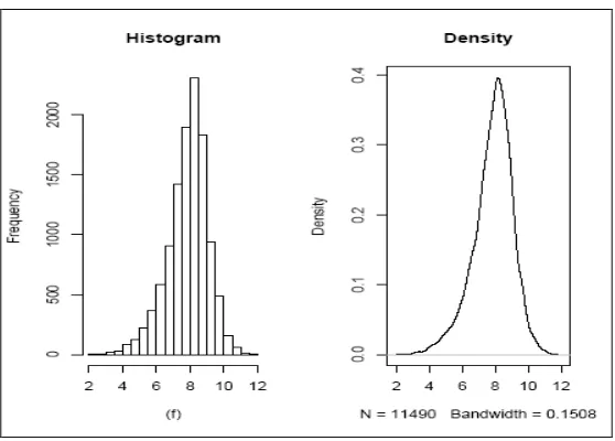
We don’t make any assumption on the form of the probability density function (pdf) of a random variable. The use of nonparametric density estimation has been used regularly to analyze incomes densities for many years, through the computation of the famous histogram. Although histogram is simple and useful for graphical depiction of the data imposes some difficulties; the discontinuity (not smooth), end points of bins and the fact that the choice of origin could be change the estimation.

The simple idea behind the histogram is at follow;

Take a rv (random variable) iid with unknown function density, then we divide the range into bins ;

= + − 1 ℎ , + ℎ", where є ( ,

(6)

[image:6.612.167.446.68.268.2]

5

Figure 1

Recurring to the definition of pdf;

( )

(

y h Y y h

)

h y

f

h − < < +

=

→ ₂ Pr

1 lim

0

,

When we want to estimate the density of Y in the interval − ℎ, + ℎ ;

ƒ, =_{2hn # 0 − ℎ, + ℎ "}1

ƒ, =_{2hn 1 2 | −}1

4 5

| ≤ ℎ

ƒ, =_{hn 1}1 1_{2 2| −}

4 5

/ℎ| ≤ 1

ƒ, =_{hn 1 7}1 −

4 5

/ℎ"

Where 7 9 =_:2 |9| ≤ 1 Is the uniform kernel function assigning 0.5 equal weights to each observation in the interval around . There are anothers kernel functions that we can mention like Epanechnikov, Biweight, Triweight, Triangular and Gaussian. The difference is the weight to the distance between to the rest of the observations.

(7)

6 ƒ, =1_{n 1 7 −}

4 5

Where K( ) =

;

7 <

∗

;

>,

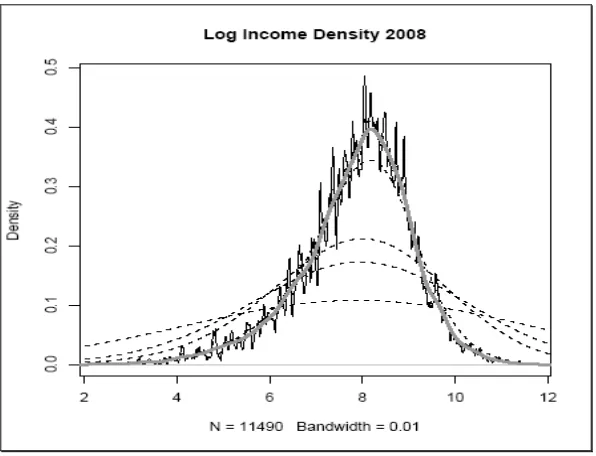
h is the bandwidth.

[image:7.612.158.456.261.489.2]

In regards to the above stated, to use Kernel Estimator we need to choose a bandwidth (h) and the kernel function. The bandwidth determines the smoothing level of the estimated density, there is a tradeoff between variance and bias when we choose ℎ. The choice of ℎ definitively is crucial, a small one reduces the bias but increases its variability, on the other side, a large bandwidth, reduces variance but increases bias, this is problematic with sparse data.

Figure 2

We can see in Figure 2 what we said before. The grey line shows the real sample income density distribution in log from the ENAHO 2008, if we increase the bandwidth the mass will be over smoothed (dotted lines), inversely, the mass will be under smoothed (strong variability) *.

(8)

7

We have to minimize MISE (Mean Integrated Squared Error) in order to choose the optimal bandwidth level.MISE is the expected value of the square of the divergence between the estimate and the true density, and it is a global measure of divergence in the sense that it is not around any particular realization of Y, MISE is definite by:

∫

( ) ( )

    ₋ =       dy y f y f E f MISE 2 ^ ^

In order to Silverman (1986) and Jae-Lee (1996), the value of h that minimizes MISE is

(

)

[

]

5 1 9 . 0 349 . 1 , min n IR Var

h= y y × , where IR = _,?@4− _,:@4 ,

(9)

8

III. Income Distribution

Usually the evolution of income distribution studies focuses to some important metrics. We can use the income mean to analyze the evolution of the position of the income density distribution. If we want to know the degree of the income’s mass concentration independently of their position, we can get the inequalities indexes. As we said before, the use of non parametric method relies in none assumption about the income density function.

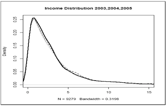
Using kernel method to estimate the income density from 2003 to 2008, in order to the exploratory character of this note we use a simple metric household’s income, we divide all the income of household’s members to the total of members, would be better use another unit of references like the “Adult Equivalence”. In the next figure we plotted the density of the income to the years 2003-2008. In Figure 3 there is a persistent movement to the left, we can conclude that the growth of the economy those years increased the mean of the income household.

(10)

9

Figure 4

[image:10.612.156.474.95.299.2]

Figure 5

(11)

10

• Indicators Summary

[image:11.612.154.474.243.366.2]

Table 1 presents the results of the statistic summary and two of the most inequality indexes used in income distribution analysis, Gini and the Theil indexes. The average growth rate of the income mean in the period analyzed was 7% while the diminishing average rate of the Gini and Theil were 0.3% and 1.4% respectively, this fact affirm the general perception commented in part I of this note about the divergence of economic growth - equality and the reasonable dissatisfaction of the population.

Table 1

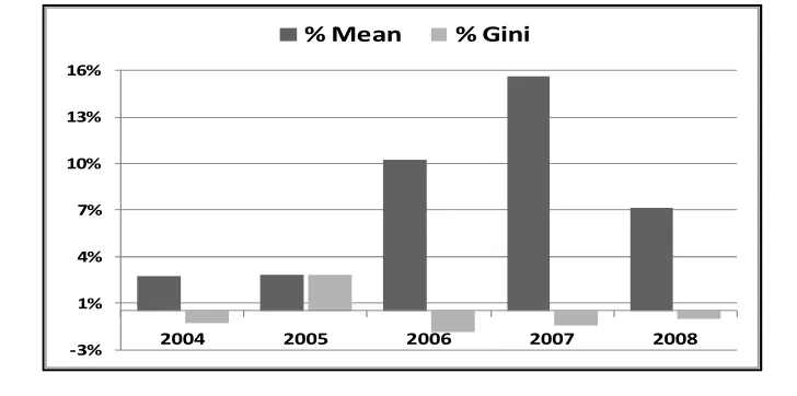
[image:11.612.123.487.511.692.2]

We plotted in figure 6 the Ginis and the growths rates of the mean of the distributions. As can be seen in Figure 6, from 2006 the falling in the inequality income rate is decreasing despite of the increasing by 15% of the mean growth rate between 2006 and 2007. The mean growth rate of the income distribution jumped from 10% in 2006 to near 16% in 2007, we could expect that this tendency will increase the equality rate but there was an inverse effect in the income distribution.

Figure 6

Year Min 1st.Quin Median Mean 3rd.Quin

Max

Gini

Theil

2003

3

943 2,088

3,350

3,902

111,359

0.5418

0.5713

2004

2

941 2,162

3,425

4,165

107,152

0.5373

0.5416

2005

9

922 2,131

3,504

4,209

182,119

0.5495

0.5824

2006

12 1,036

2,365

3,844

4,687

131,468

0.5421

0.5498

2007

10 1,206

2,834

4,424

5,422

115,486

0.5370

0.5279

2008

10 1,346

3,030

4,716

5,776

113,418

0.5340

0.5268

-3% 1% 4% 7% 10% 13% 16%

2004 2005 2006 2007 2008

(12)

11

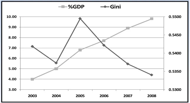
[image:12.612.146.468.217.392.2]

We plotted the evolutions of GDP growth rate versus the of the Gini index in Figure 7. The GDP growth in a sustained way, jumping from S/. 139 Billion of Nuevos soles in 2003 to S/. 192 Billion in 2008* despite of the evolution of inequality income, even though since 2005 the inequality has been diminishing but not in equal magnitude of the GDP growths as we commented before.

Figure 7

• Robustness of Indicators

The bootstrap method introduced in Efron (1979) is a very general resampling procedure for estimating the distributions based on independent observation. The boostrap method is being accepted as an alternative to the asymptotic methods. Being better than some others asymptotic methods such as the traditional Edgeworth expansion and the Normal approximation. With bootstrap method the basic sample is treated as the population and a Monte Carlo process is conducted on it. This is done by randomly drawing a large number of resamples of equal size of the original sample with replacement, these new samples could include some of the original data more than once and some not included. The elements of these resample vary slimly and we could calculate slightly different values of some statistic estimator.

*Central Bank of Peru: www.bcrp.gob.pe

0.5300 0.5350 0.5400 0.5450 0.5500

3.00 4.00 5.00 6.00 7.00 8.00 9.00 10.00

2003 2004 2005 2006 2007 2008

(13)

12

[image:13.612.139.494.310.438.2]

The objective of this note was analyze and calculate the inequality indexes of the incomes households from 2003 to 2008, in order to assure if these indexes increased or decreased we used bootstrapping techniques. The surveys hasn’t a complete panel structure; there is not the same sample year by year, so we need some replication statistical technique allow to have good variability’s metrics to some estimator, in this case the Gini index. Using the samples of the ENAHO income distribution 2003-2008 we replicates each distribution with replace in order to calculate the variability sample of the Gini’s indexes, we did a Montecarlo Resampling Method to obtained the new samples. We evaluated the null hypothesis of no variability on inequality of the income distribution.

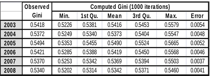
Table 2

In Table 2 we compare the Gini’s coefficients observed in the original sample with those computed with bootstrapping techniques with 1000 iterations. As we can see the coefficients of inequality have been estimated with high accuracy, it can be explained because the number of iterations, we can confirm this with the low levels of the errors.

The main idea of this part of the note is to have some formal indicator of weather the observed distributions indeed changed from year to year or if the viewed shifts indexes were not significant in a statistical sense. We decided to perform two nonparametric tests for equality of distribution functions paired years.

One of them was proposed by Mann, Whitney and Wilcoxon (MWW), the MWW test. Normal distribution of data is not necessary for this test. It’s a nonparametric test based on the idea that the equality of two distributions can be inferred from the rank that their items take within the combined distribution. Formally, suppose there are to distributions F(x) and G(y) defined over

Min. 1st Qu. Me a n 3rd Qu. Ma x. Error 2003 0.5418 0.5226 0.5381 0.5416 0.5453 0.5579 0.0054

2004 0.5372 0.5249 0.5340 0.5373 0.5404 0.5547 0.0048

2005 0.5494 0.5353 0.5455 0.5490 0.5524 0.5665 0.0052

2006 0.5421 0.5285 0.5388 0.5419 0.5450 0.5568 0.0046

2007 0.5370 0.5253 0.5342 0.5369 0.5394 0.5503 0.0037

2008 0.5340 0.5202 0.5314 0.5342 0.5371 0.5460 0.0041

Observe d Gini

(14)

13

of two random variables X= X1,…,Xm, and Y= Y1,…,Yn. Adding the samples, we will have n+m

elements. Being T the sum of the ranks of the elements of Y among the n+m items of the combined sample, and define the test statistic;

2 ) 1

( +

− =T n n

U the Test is defined by;

∑ ∑

₌ ₌

= m j

n i Zij U

1 1

Z

ij

=

1 ,

if

X

i

<

Y

j

0, otherwise

If the two samples are enough large and we can’t reject the A equality hypothesis the following statistic is distributed as a N(0,1) random variable;

U

Var

U

_

−

Where 12 ) 1 ( 2 _ + + =

= mn and Var mn m n

U U

We can find U’s tables in many statistics texts. If we use it the column number should be the number of the larger sample and the row number should be of the smaller one. On the other hand, if we use the Z value and it doesn’t equal or exceed the critical Z value of 1.96 (95% two tailed test), then you can assume that the null hypothesis is correct and there is no difference between samples. However, if Z exceeds 1.96 then you have evidence to reject the null hypothesis. Maybe it is more convenient observing the p-value as we did in this note. Therefore, once the values of T and U are found, it is straightforward to test the null hypothesis Ho: F(x)=G(y).

The other is the well known Kolmogorov-Smirnov test. Technically, suppose that a first sample

X1,...,Xm of size m has distribution with c.d.f. F (x) and the second sample Y1,...,Yn of size n has distribution with c.d.f. G(x) and we want to test

A : C = D EF. A : C ≠ D

If C_I and D₄ are corresponding empirical c.d.f ‘s then the contrast statistic is;

J

II

= <

_IK4I4

>

.@

(15)

14

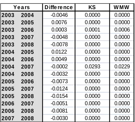
Table 3 shows the results of the equality tests for pairs of years, in column 2 we show the differences of the Gini’s indexes, column 3 and 4 displays the p-values of the null hypothesis that the true location shift is equal to 0, checking up the p values we could accept the alternative hypothesis that the true location shift is not equal to 0, confirming that the changes in the income distribution year from year have statistical significant outcomes.

Table 3

D iffe re nce KS W MW 2003 2004 -0.0046 0.0000 0.0000

2003 2005 0.0076 0.0000 0.0000

2003 2006 0.0003 0.0001 0.0006

2003 2007 -0.0048 0.0000 0.0000

2003 2008 -0.0078 0.0000 0.0000

2004 2005 0.0122 0.0000 0.0000

2004 2006 0.0049 0.0000 0.0000

2004 2007 -0.0002 0.0293 0.0229

2004 2008 -0.0032 0.0000 0.0000

2005 2006 -0.0073 0.0000 0.0000

2005 2007 -0.0124 0.0000 0.0000

2005 2008 -0.0154 0.0000 0.0000

2006 2007 -0.0051 0.0000 0.0000

2006 2008 -0.0081 0.0000 0.0000

2007 2008 -0.0030 0.0000 0.0000

[image:15.612.202.430.224.431.2]

(16)

15

IV. Final Comments

(17)

16

References

Sosa Escudero, Walter and Leonardo Gasparini (2000). “ A note on the statistical significance of changes in inequality”. Económica, Vol. XLVI(1): 111-122.

The World Bank Country Profiles (2007)

Gasparini (2004). Different lives: inequality in Latin America and the Caribbean. Breaking with History ?, The World Bank.