Stochastic Analysis of Low Cost Single Frequency GPS Receivers

ISSN Online: 2150-8526 ISSN Print: 2150-850X

Stochastic Analysis of Low-Cost Single-Frequency

GPS Receivers

Mohamed Elsayed Elsobeiey

Department of Hydrographic Surveying, Faculty of Maritime Studies, King Abdulaziz University, Jeddah, Kingdom of Saudi Arabia

Abstract

Typically, dual-frequency geodetic grade GNSS receivers are utilized for positioning applications that require high accuracy. Single-frequency high grade receivers can be used to minimize the expenses of such dual-frequency receivers. However, user has to consider the resultant positioning accuracy. Since the evolution of low-cost sin-gle-frequency (LCSF) receivers is typically cheaper than sinsin-gle-frequency high grade receivers, it is possible to obtain comparable positioning accuracy if the correspond-ing observables are accurately modelled. In this paper, two LCSF GPS receivers are used to form short baseline. Raw GPS measurements are recorded for several con-secutive days. The collected data are used to develop the stochastic model of GPS observables from such receivers. Different functions are tested to determine the best fitting model which is found to be 3 parameters exponential decay function. The new developed model is used to process different data sets and the results are compared against the traditional model. Both results from the newly developed and the tradi-tional models are compared with the reference solution obtained from dual-fre- quency receiver. It is shown that the newly developed model improves the root- mean-square of the estimated horizontal coordinates by about 10% and improves the root-mean-square of the up component by about 39%.

Keywords

Single-Frequency Receiver, Stochastic Analysis, Precise Point Positioning

1. Introduction

Typically, differential GPS based on carrier phase observables is the first alternative for users seeking centimeter level accuracy [1]. However, a major disadvantage of such technique is its dependency on corrections or data from a reference receiver, i.e. at least two dual-frequency receivers are required [2] [3]. Commercial GPS receivers vary

ac-How to cite this paper: Elsobeiey, M.E. (2016) Stochastic Analysis of Low-Cost Single- Frequency GPS Receivers. Positioning, 7, 91- 100. http://dx.doi.org/10.4236/pos.2016.73009

Received: July 16, 2016 Accepted: August 28, 2016 Published: August 31, 2016

Copyright © 2016 by author and Scientific Research Publishing Inc. This work is licensed under the Creative Commons Attribution International License (CC BY 4.0).

cording to their receiving capabilities. With availability of precise ephemerides and termination of Aelective Availability (SA), it becomes possible to obtain position accu-racy comparable to that which can be obtained from differential techniques using single receiver. This technique is well known as “Precise Point Positioning” (PPP). In PPP, the undifferenced carrier phase and pseudoranges on both frequencies are utilized to form the first-order ionosphere-free linear combination to eliminate the first-order ionos-phere-delay effect. PPP was first introduced by researchers at the Jet Propulsion Labor-atory [4]. However, to achieve such accuracy all errors and biases must be rigorously modelled [5]. Few millimeters accuracy is achievable if precise orbit and clock correc-tions are applied [6]. For more details about the PPP technique and the corresponding error modelling one can refer to [4] [7] [8].

Unlike dual-frequency receivers, however, ionosphere delay represents a major chal-lenge for single-frequency receivers. There are two main techniques to account for io-nosphere delay in case of single-frequency receivers [9]. The first technique is to use ionosphere models to correct for the ionosphere delay. These models may be empirical models such as Klobuchar model, which can account for up to 60% of the delay at mid- latitudes [3]. Klobuchar model coefficients are transmitted in the navigation message and can be improved by extending the eight parameters original Klobuchar model to ten-parameters to account for the ionosphere variation during the night time [10]. Corrections from regional or global network may be estimated and then applied to sin-gle-frequency receivers [11]. An example for the global ionosphere corrections, which is used in this paper, is the Global Ionosphere Maps (GIMs) produced by the Interna-tional GNSS service (IGS). Another option for real-time ionosphere delay correction is to broadcast ionosphere corrections from Space Based Augmentation Systems (SBAS)

[12] and [13].

The second technique to account for ionosphere delay is to form ionosphere-free li-near combination using both code and carrier phase observations on L1 from the sin-gle-frequency receiver. This technique is based on the Group and Phase Ionosphere Ca-libration (GRAPHIC) [9] [14]-[16].

In addition to the low-cost, high sensitivity single-frequency receiver are able to ac-quire signals with low decibel watt (dBW) [17]. Standalone relative localization system can be established using low-cost receivers to monitor the relative motion of the neighboring notes rather than the absolute position of each node [18]. Ambiguity reso-lution, on the other hand, can be achieved for single-frequency data [19]. Sub-cm and few centimeters accuracy levels can be achieved for horizontal and vertical directions, respectively, if 10 minutes of accumulated data are used [20]. Moreover, geodetic grade antenna can be used with LCSF receivers to improve its performance [21].

2. Mathematical Model

The mathematical models for undifferenced pseudorange and carrier phase measure-ments can be written as follows [22] [23]:

(

)

1 1 1

r s

C

C = +ρ c dt −dt + + +T I e (1)

(

)

1 1 1 1 1

r s

N

c dt dt T I

ρ+ λ εΦ

Φ = − + − + + ₍₂₎

where, C1 is the pseudorange (code) measurements on L1; Φ1 is the carrier phase

measurements on L1 scaled to distance (m); dt dts, r are the satellite and receiver clock

errors, respectively; λ1 is the L1 carrier phase wavelength; N1 is the L1 integer

am-biguity; c is the speed of light in vacuum (m/sec); ρ is the true geometric distance between satellite antenna phase center and receiver antenna phase center at reception time (m); I1 is the L1 ionosphere delay (m); T is the slant tropospheric delay (m); and

1, 1

C

e ε_Φ are the unmodeled errors including residual orbital error, hardware delay,

noise and multipath effect.

3. Stochastic Model

The final solution of least-squares of positioning model (Equations (1) and (2)) does not depend only on the mathematical formulation of the unknowns, but also depend on the statistical representation of the observations and unknowns. The observations sto-chastic properties are reflected in the weight matrix of observations, which includes the corresponding relative and absolute accuracies. The GPS signal’s power can be used as a measure of the signal quality. For example, the signal-to-noise ratio and carrier-to- noise power density ratio can be used as a measure of the GPS signal power and used to weight different signals [24]. Elevation angle, on the other hand, can be used to diffe-rentiate between the data quality from each satellite. The relationship between the pre-cision of observations and the corresponding satellite elevation can be expressed in sine or cosine function as seen in Equation (3).

( )

1

, is the satellite elevation angle sin el el

σ = ₍₃₎

Stochastic properties of GPS receiver’s signals can be determined through the cali-bration process. Typically, receiver noise can be examined using zero baseline [25]. However, short baseline test can be used to evaluate the full system noise (GPS antenna and receiver) by collecting data over two consecutive days. In this case, the combina-tion of the double-differenced residuals of one day will contain both effects of multi-path (if it exists) and system noise. Because every sidereal day the multimulti-path effect is repeated, differencing the double-differenced combination over two consecutive days cancels out the multipath effect and leaves the system noise only [3]. By differencing the double-differenced combination between two consecutive days the system noise is doubled. To obtain the standard deviation of the double-differenced system noise, the system noise should be divided by 2.

the carrier phase measurements [5]. The noise level of the carrier phase measurements is approximately 1% of that of the pseudorange measurements. Hence, the carrier phase noise and multipath can be neglected in comparison with those of pseudorange mea-surements. The C/A-code pseudorange noise can be computed as follows:

1 1 21 1N1 C1

C − Φ = I −λ +e (4)

Equation (4) can be differenced between the two receivers forming between receiver single difference, which sufficiently cancels out the ionosphere delay. The remaining terms include the integer ambiguity, hardware delay, system noise and multipath effect. Since the multipath effect is repeated each sidereal day, it can be sufficiently removed by differencing over two consecutive days. The integer ambiguity number is constant as long as the receiver tracks the satellite and hardware delay is stable over several days. As such, both can be removed from the combination by subtracting the first value of the time series. At this stage, we have only the differenced system noise in the time series. The differenced combination can be divided into bins based on the satellite elevation angle, and the best fitted mathematical function for observations standard deviation can be determined.

4. Field Test

To investigate the stochastic properties of LCSF receiver, two u-box New-7P GPS re-ceivers are used to form short baseline. The short baseline is fixed on the roof top of Faculty of Maritime Studies (FMS) building beside a base station established using Topcon GR3 GNSS receiver (used as a reference). GPS data are collected at sampling frequency of 1 Hz from both single-frequency and dual-frequency receiver. The col-lected data are used to examine the noise level of single-frequency receivers. The de-veloped model is used to process new session of GPS data collected using the same sin-gle-frequency receivers.

5. Results and Discussion

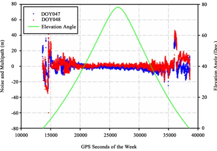
The single frequency data collected for two consecutive days is used to compute code- carrier observable (Equation (4)) for both receivers. The new observable from the two receivers is used to form between-receiver single-difference combination to remove the ionosphere delay. However, the resultant combination is affected by the multipath ef-fect. Since the multipath effect is repeatable every sidereal day, subtracting such com-bination from two consecutive days will successfully remove the multipath effect. It should be noted here that the sidereal day is 23 hours 56 minutes and 4 seconds which is less than the solar day by 3 minutes and 56 seconds (i.e., 256 Seconds). Hence, to re-move the multipath effect, the second day series should be shifted by 236 seconds. Fig-ure 1 shows noise and multipath effect for PRN06, as an example, for DOY047 and DOY048 before applying the time shift while Figure 2 shows noise and multipath effect after applying time shift of 236 seconds.

Figure 1. Multipath and Noise for PRN06 During DOY047 and DOY048, 2016.

Figure 2. Multipath and noise for PRN06 during DOY047 and DOY048, 2016. After applying 236 seconds time shift to DOY048.

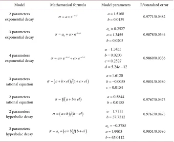
mathematical function that fits the data. Different techniques are applied to determine the best model that fits the data including 2 parameters exponential decay function, 3 parameters exponential decay function, 4 parameters exponential decay function, 3 pa-rameters rational equation, 2 papa-rameters rational equation, 2 papa-rameters hyperbolic decay function, and 3 parameters hyperbolic decay function. Table 1 summarizes the fitting parameters for all tested models.

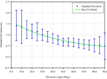
Figure 3 shows that the standard deviation of C/A code is about 0.5 m and 1.5 m at 90° _{and 05}° _{elevation angles, respectively. These results makes sense for single-frequency}

receiver if Trimble R7 GNSS receiver’s model has corresponding values of 0.2 m and 0.7 m at elevation angles of 90° _{and 05}°_{, respectively [5]. To test the developed model,}

new raw data are collected using the same single-frequency receivers in addition to dual-frequency data of the base station which is used as a reference. The mathematical model used as in Equations (1) and (2). The ionosphere delay is modelled using the IGS GIMs. Satellite orbit and clock corrections are accounted for using the corresponding IGS final products. Tropospheric delay is modelled using the Global Pressure and Temperature 2 (GPT2) model [26]. ECMWF’s “European Centre for Medium-Range Weather Forecasts” Vienna mapping function 1 (VMF1) is used for mapping tropo-spheric delays to the elevation angle of each satellite [27] [28]. All remaining errors, in-

Table 1. Summary of fitted models parameters.

Model Mathematical formula Model parameters R2_{/standard error}

2 parameters

exponential decay σ= ×a e− ×b el

1.5168 0.0139 a b = = 0.9771/0.0482 3 parameters

exponential decay 0 e

b el

a a

σ_{= + ×} − ×

0 0.2527 1.3455 0.0203 a a b = = = 0.9878/0.0344 4 parameters

exponential decay σ= ×a e− ×b el+ ×c e− ×d el

1.3455 0.0203 0.2527 5.24 12 a b c d e = = = = − 0.9869/0.0356 3 parameters

rational equation σ =(a+ ×b el) (1+ ×c el)

1.6120 0.0058 0.0154 a b c = = − = 0.9851/0.0380 2 parameters

rational equation σ =1(a+ ×b el)

0.5844 0.0155 a b = = 0.9767/0.0475 2 parameters

hyperbolic decay σ=(a b× ) (b+el)

1.7111 37.7312 a b = = 0.9767/0.0475 3 parameters

hyperbolic decay σ=a0+(a b× ) (b+el)

0 0.3785 1.9905 65.0112 a a b = − = = 0.9851/0.0380

Figure 3. The best fitted model for the relationship between elevation angle and standard deviation.

cluding ocean loading, Earth tides, carrier phase windup, relativity, and sagnac effect are accounted for using existing models [29]. The processing is performed using two different models for observations weights. The first model is the traditional model (Eq-uation (3)), which is used for most GNSS processing software by default. The second model is the developed model (3 parameters exponential decay function), which devel-oped based on our experiment. Our results showed that the develdevel-oped model improves the solution of Easting, Northing, and Up components. Moreover, using the dual-fre- quency solution as a reference, the uncertainty of the estimated coordinates using both (traditional and developed) models are at 39% confidence level then transformed to 95% confidence level as follows [30]:

(

) (

)

, ,

2 1

39%

ˆ ˆ ˆ ˆ

n

REF T D REF T D

i i

D i

N N E E

THE

n

=

− + −

=

∑

2 2

95% 2.44 39%

D D

THE = THE (6)

(

)

1 1

39%

ˆ ˆ

n

REF T D i

D i

U U

TVE

n

=

−

=

∑

1 1

95% 1.96 39%

D D

TVE = TVE (8)

where 2 39%

D

THE represents the total 2D horizontal error of Northing and Easting

posi-tion errors at 39% confidence level, ˆ

REF

N the easting coordinate of the reference

de-veloped models, ˆ

REF

E is the Easting coordinate of the reference solution, Eˆ_{T D,} is the

Easting single-frequency position using the traditional or the developed models, n is the total number of epochs, 2

95%

D

THE is the 2D total horizontal error of Northing and

Easting position error at 95% confidence level, 1 39%

D

TVE represents the total 1D vertical

error of the Up component at 39% confidence level, and 1 95%

D

TVE represents the total

1D vertical error of the Up component at 95% confidence level. Table 2 summarizes the THE and TVE values at 39% and 95% confidence levels.

Table 2 shows that the total horizontal error is 5.410 m and 4.880 m for the tradi-tional and the developed models at 95% confidence level, respectively. This means that an improvement by about 10% in the horizontal component can be achieved by the de-veloped model. The vertical component, on the other hand, shows that the total vertical error is 1.960 m for traditional model compared with 1.203 m for the developed model which means an improvement of 39% in the vertical component.

6. Conclusion

In this paper, we investigated the stochastic properties of low-cost-single-frequency re-ceivers. The main objective is to develop stochastic model to improve the positioning performance of such receivers. Raw GPS measurements are collected using two low-cost single-frequency GPS receivers fixed to form short baseline. A third dual-frequency receiver is used as a reference to evaluate the performance of low-cost single-frequency receivers. Between receivers, single difference is formed using the code-carrier combination from both receivers and the ambiguity term and hardware delay constants are removed from each satellite pass. The resultant combination is dif-ferenced over two consecutive days to eliminate the multipath effect. The final noise is used to develop the relationship between the satellite elevation angle and signal stan-dard deviation. Different functions are tested to determine the best model that fits such relationship. It is found that the 3 parameters exponential decay function is the best fit model. The developed model is used to process different data sets. Both solutions from the traditional (sine function) and the developed models are compared with the refer-ence solution. It is shown that the developed model can improve the accuracy of the es-timated coordinates by about 10% and 39% for the horizontal and up components,

Table 2. Summary statistics of the developed model compared with the traditional model.

Error Parameter Total Error (m) % Improvement

Traditional Model Developed Model

2 39%

D

THE 2.220 2.000

2 95%

D

THE 5.410 4.880 9.9%

1 39%

D

TVE 1.000 0.614

1 95%

D

respectively. These results can be considered significant to improve the performance of low-cost single-frequency receivers.

References

[1] Grewal, M.S., Weill, L.R. and Andrews, A.P. (2007) Global Positioning Systems, Inertial Navigation, and Integration. 2nd Edition, Wiley-Interscience, Hoboken.

http://dx.doi.org/10.1002/0470099720

[2] El-Rabbany, A. (2006) An Autonomous GPS Carrier-Phased-Based System for Precision Navigation. Intelligent Transportation Systems Conference, 2006. ITSC’06, 17-20 Septem-ber 2006. http://dx.doi.org/10.1109/itsc.2006.1706837

[3] El-Rabbany, A. (2006) Introduction to GPS: The Global Positioning System. 2nd Edition, Artech House Mobile Communications Series, Artech House, Boston, xiv, 210 p.

[4] Zumberge, J.F., Heflin, M.B., Jefferson, D.C., Watkins, M.M. and Webb, F.H. (1997) Precise Point Positioning for the Efficient and Robust Analysis of GPS Data from Large Networks.

Journal of Geophysical Research: Solid Earth, 102, 5005-5017.

http://dx.doi.org/10.1029/96JB03860

[5] Elsobeiey, M. and El-Rabbany, A. (2010) On Stochastic Modeling of the Modernized Global Positioning System (GPS) L2C Signal.Measurement Science and Technology, 21, 055105.

http://dx.doi.org/10.1088/0957-0233/21/5/055105

[6] Kouba, J. and Héroux, P. (2001) Precise Point Positioning Using IGS Orbit and Clock Products.GPS Solutions, 5, 12-28. http://dx.doi.org/10.1007/PL00012883

[7] Witchayangkoon, B. (2000) Elements of Gps Precise Point Positioning, in Department of Spatial Information Science and Engineering. The University of Maine, Orono.

[8] Bisnath, S. and Gao, Y. (2009) Precise Point Positioning: A Powerful Technique with a Promising Future. GPS World, 20, 43-50.

[9] Cai, C., Liu, Z. and Luo, X. (2013) Single-Frequency Ionosphere-Free Precise Point Posi-tioning Using Combined GPS and GLONASS Observations.The Journal of Navigation, 66, 417-434. http://dx.doi.org/10.1017/S0373463313000039

[10] Wang, N., Yuan, Y., Li, Z. and Huo, X. (2016) Improvement of Klobuchar Model for GNSS Single-Frequency Ionospheric Delay Corrections.Advances in Space Research, 57, 1555- 1569. http://dx.doi.org/10.1016/j.asr.2016.01.010

[11] Wübbena, G., Schmitz, M. and Bagge, A. (2005) PPP-RTK: Precise Point Positioning Using State-Space Representation in RTK Networks. Proceedings of ION GNSS, Long Beach, 13-16 September 2005, 2584-2594.

[12] Hofmann-Wellenhof, B., Lichtenegger, H. and Wasle, E. (2008) GNSS—Global Navigation Satellite Systems: GPS, GLONASS, Galileo, and More. Springer, Wien, New York, xxix, 516 p.

[13] Arbesser-Rastburg, B. (2002) Ionospheric Corrections for Satellite Navigation Using EGNOS. Proceedings of 27th URSI General Assembly, Maastricht, 17-24 August 2002. [14] Shi, C., Gu, S., Lou, Y. and Ge, M. (2012) An Improved Approach to Model Ionospheric

Delays for Single-Frequency Precise Point Positioning.Advances in Space Research, 49, 1698-1708. http://dx.doi.org/10.1016/j.asr.2012.03.016

[15] Sterle, O., Stopar, B. and Pavlovčič Prešeren, P. (2015) Single-Frequency Precise Point Posi-tioning: An Analytical Approach.Journal of Geodesy, 89, 793-810.

http://dx.doi.org/10.1007/s00190-015-0816-2

Frequency GNSS Positioning. GPS Solutions, 15, 139-147.

http://dx.doi.org/10.1007/s10291-010-0177-5

[17] Schwieger, V. (2007) High-Sensitivity GPS—The Low Cost Future of GNSS. FIG Working Week, Hong Kong, 13-17 May 2007, 1-16.

[18] Hedgecock, W., Maroti, M., Sallai, J., Volgyesi, P. and Ledeczi, A. (2013) High-Accuracy Differential Tracking of Low-Cost GPS Receivers. Proceeding of the 11th Annual

Interna-tional Conference on Mobile Systems, Applications, and Services, Taipei, 25-28 June 2013,

221-234. http://dx.doi.org/10.1145/2462456.2464456

[19] Odijk, D., Teunissen, P. and Zhang, B. (2012) Single-Frequency Integer Ambiguity Resolu-tion Enabled GPS Precise Point PosiResolu-tioning. Journal of Surveying Engineering, 138, 193- 202. http://dx.doi.org/10.1061/(ASCE)SU.1943-5428.0000085

[20] Odijk, D., Teunissen, P.G. and Khodabandeh, A. (2014) Single-Frequency PPP-RTK: Theory and Experimental Results. In: Rizos, C. and Willis, P., Eds., Earth on the Edge: Sci

-ence for a Sustainable Planet, Springer, Berlin, 571-578.

http://dx.doi.org/10.1007/978-3-642-37222-3_75

[21] Takasu, T. and Yasuda, A. (2008) Evaluation of RTK-GPS Performance with Low-Cost Sin-gle-Frequency GPS Receivers. Proceedings of International Symposium on GPS/GNSS, Tokyo, 11-14 November 2008, 852-861.

[22] Kleusberg, A. and Teunissen, P.J.G. (1998) GPS for Geodesy. 2nd Edition, Vol. 14, Springer, Berlin, 650 p.

[23] Leick, A. (2004) GPS Satellite Surveying. 3rd Edition, Vol. 24, John Wiley, Hoboken, 435 p. [24] Özlüdemir, M.T. (2004) The Stochastic Modeling of GPS Observations. Turkish Journal of

Engineering and Environmental Sciences, 28, 223-232.

[25] Nolan, J., Gourevitch, S. and Ladd, J. (1992) Geodetic Processing Using Full Dual Band Observables. Proceedings of the 5th International Technical Meeting of the Satellite

Divi-sion of the Institute of Navigation (ION GPS 1992), Albuquerque, 16-18 September 1992,

1033-1041.

[26] Lagler, K., Schindelegger, M., Böhm, J., Krásná, H. and Nilsson, T. (2013) GPT2: Empirical Slant Delay Model for Radio Space Geodetic Techniques. Geophysical Research Letters, 40, 1069-1073. http://dx.doi.org/10.1002/grl.50288

[27] Boehm, J., Niell, A., Tregoning, P. and Schuh, H. (2006) Global Mapping Function (GMF): A New Empirical Mapping Function Based on Numerical Weather Model Data.

Geophysi-cal Research Letters, 33, Article ID: L07304. http://dx.doi.org/10.1029/2005gl025546

[28] Boehm, J., Werl, B. and Schuh, H. (2006) Troposphere Mapping Functions for GPS and Very Long Baseline Interferometry from European Centre for Medium-Range Weather Forecasts Operational Analysis Data. Journal of Geophysical Research: Solid Earth, 111, Article ID: B02406. http://dx.doi.org/10.1029/2005jb003629

[29] Kouba, J. (2009) A Guide to Using International GNSS Service (IGS) Products.

http://igscb.jpl.nasa.gov/igscb/resource/pubs/GuidetoUsingIGSProducts.pdf

[30] El-Diasty, M. and Elsobeiey, M. (2015) Precise Point Positioning Technique with IGS Real- Time Service (RTS) for Maritime Applications. Positioning, 6, 71-80.

Submit or recommend next manuscript to SCIRP and we will provide best service for you:

Accepting pre-submission inquiries through Email, Facebook, LinkedIn, Twitter, etc. A wide selection of journals (inclusive of 9 subjects, more than 200 journals)

Providing 24-hour high-quality service User-friendly online submission system Fair and swift peer-review system

Efficient typesetting and proofreading procedure

Display of the result of downloads and visits, as well as the number of cited articles Maximum dissemination of your research work