Recent Evidence on Residential Electricity Consumption Determinants: A Panel Two Stage Least Squares Analysis, 2001 2005

(1)

Munich Personal RePEc Archive

Recent Evidence on Residential

Electricity Consumption Determinants:

A Panel Two-Stage Least Squares

Analysis, 2001-2005

Cebula, Richard and Herder, Nate

Jacksonville University, Armstrong Atlantic State University

28 February 2009

Online at

https://mpra.ub.uni-muenchen.de/56741/

(2)

RECENT EVIDENCE ON RESIDENTIAL ELECTRICITY

CONSUMPTION DETERMINANTS: A PANEL TWO-STAGE

LEAST SQUARES ANALYSIS, 2001-2005

Richard J. Cebula and Nate Herder

Abstract. This empirical study seeks to provide evidence identifying key factors that have influenced per residential customer electricityconsumption in the U.S. during recent years. This empirical analysis takes the form of P2SLS (panel two-stage least squares) estimations. State-level data are adopted for the five-year period from 2001 through 2005. The P2SLS findings indicate that the annual consumption of electricity per residential customer is an increasing

function of the annual number of cooling degree days, real per capita personal disposable income, and the real unit price of natural gas. Annual per residential customer electricity consumption is also found to be a decreasing function of the real unit price of electricity and the extent of usage of natural gas for residential heating, as well as the degree to which each state has pursued energy efficiency policies. Finally, said consumption is also found to be positively a function of a control variable measuring peak summer electricity generating capacity.

(3)

RECENT EVIDENCE ON DETERMINANTS OF PER

RESIDENTIAL CUSTOMER ELECTRICITY CONSUMPTION

IN THE U.S.: 2001-2005

Abstract. This empirical study seeks to provide evidence identifying key factors that have influenced per residential customer electricityconsumption in the U.S. during recent years. This empirical analysis takes the form of P2SLS (panel two-stage least squares) estimations. State-level data are adopted for the five-year period from 2001 through 2005. The P2SLS findings indicate that the annual consumption of electricity per residential customer is an increasing

function of the annual number of cooling degree days, real per capita personal disposable income, and the real unit price of natural gas. Annual per residential customer electricity consumption is also found to be a decreasing function of the real unit price of electricity and the extent of usage of natural gas for residential heating, as well as the degree to which each state has pursued energy efficiency policies. Finally, said consumption is also found to be positively a function of a control variable measuring peak summer electricity generating capacity.

Keywords: Residential electricity consumption, Electricity prices, Natural gas prices, Income, Cooling degree days, Natural gas usage, Energy efficiency policies

I. Introduction

The June 22, 2009 issue of National Geographic was devoted entirely to the topic

“Energy for Tomorrow.” Among the numerous timely issues considered at length in this publication is an expected massive (“nearly 50 percent”) growth in the demand for energy over the next 21 years and the concurrent potential massive rise in CO2 and other greenhouse

emissions that are allegedly heating our planet and putting us on a path that could raise the mean global temperature by as much as six degrees Celsius by 2030 (National Geographic Society, 2009, p.7). These concerns appear consistent with those of the International Energy Agency (2008, p. 4), where world primary energy demand is predicted to rise by roughly 1.6 percent annually (on average). Also noted is the critical role of coal being used to generate electricity. For example, it is observed that daily“Some 14,000 tons of coal fuel Utah’s Hunter Power Plant,

which feeds the grid in the burgeoning West” (National Geographic Society, 2009, p. 9). The

advantages of a “Smart Grid, which matches supply to demand, thereby elevating efficiency and

diminishing the need for more power plants is also discussed, along with its projected cost for just the U.S. of $400 billion (National Geographic Society, 2009, p. 30). Numerous other issues are raised, including how we can better do a better job of conservation and whether we can

(4)

From a narrower and thus somewhat different perspective, namely, that of the American Society of Civil Engineers (2009, p. 134), it is argued that “The U.S. generation and transmission [of electricity] is at a critical point requiring substantial commitment in new-generation

investment to improve efficiencies in the existing generation [of electricity], and investment in new transmission and distribution systems.” The ASCE (2009, p. 134) has noted that electricity demand has increased about 25 percent since 1990, during which time construction of new transmission facilities decreased by roughly 30 percent. Overall, the ASCE (2009, p. 134)

observes that “ The transmission and distribution system has become congested because growth in electricity demand and investment in new generation facilities have not been matched by

investment in new transmission facilities.” Finally, the ASCE (2009, p. 134) warns that massive investment in generation, transmission, and distribution facilities are needed in the next two decades in order to avert a trend towards increasingly serious congestion, shortages, and bottlenecks in electricity consumption in the U.S.

Under the appropriate rubric of environmental economics as well as regional economics, an extensive empirical literature concerned with energy consumption has developed during the last few decades. A significant component of this literature is concerned with the consumption of electricity, including the residential consumption thereof (Taylor, 1975; Halvorsen, 1975, 1978; Garbacz, 1983; Dubin and McFadden, 1984; Bohi, 1984; Dodgson, Millward, and Ward, 1990; Branch, 1993; Harris and Liu, 1993; Sailor and Munoz, 1997; Joskow, 1997; Yan, 1998; Henley and Peirson, 1998; Holtedahl and Joutz, 2004; Kamerschen and Porter, 2004; Halstead, Stevens, Harper, and Hill, 2004; Moral-Carcedo and Vicens-Otero, 2005; Zachariadis and Pashourtidou, 2007; Horowitz, 2007). The residential consumption of electricity in the U.S. will presumably continue to rise as the population continues to increase, especially if claims of global warming are correct (ASCE, 2009; Harris and Liu, 1993; Energy Information Administration, 2006), making it all the more important for both policymakers and energy firms to understand the factors influencing that consumption.

Clearly, a sound knowledge of systematic contemporary determinants of residential electricity consumption is invaluable to policymakers and private sector decision makers in the electricity industry, given the apparent investment and infrastructure challenges facing the U.S. in coming years. Accordingly, the present study seeks to identify key economic factors and other conditions that have influenced the consumption of electricity per residential customer in the U.S. during recent years. Among other things, the study investigates the impact on this measure of residential electricity consumption of the degree to which each state has pursued energy efficiency policies. Thus, the question of whether state energy-efficiency policies work is integrated into the present analysis.

Unlike most previous studies, this study uses a state-level panel data set for the period 2001 through 2005. By focusing on this time period, the evidence provided in this study is

(5)

II. The Initial Framework

The analysis in principle initially follows Halvorsen (1975), Dubin and McFadden (1984), Dodgson, Millward, and Ward (1990), Harris and Liu (1993), Holtedahl and Joutz (2004),

Kammerschen and Porter (2004), Moral-Carcedo and Vicens-Otero (2005), Zachariadis and Pashourtidou (2007), Horowitz (2007) and others in modeling residential electricity consumption as largely a function of a number of essentially demand-driven forces. The measurement of residential electricity consumption is undertaken on a per residential customer basis.

The eclectic model of residentialelectricity consumption is initially expressed as follows:

RCPCjt = f(CDDjt, ELPRjt, INCjt, NATGASPRjt, NATGASHEATjt) (1)

where (data source in parentheses):

RCPCjt = the total consumption of residential electricity (kilowatt hours) per residential

customer in state j in year t, measured as the ratio of total residential electricity consumption in state j in year t to the total number of residential customers in state j in year t (Electric Power Annual-State Data Table, 2008);

CDDjt = total annual number of cooling degree days in state j in year t (National Climatic Data Center, 2008);

ELPRjt = the average real price of residential electricity in state j in year t, measured in cents per kilowatt hour (Electric Power Annual-State Data Table, 2008) scaled by the cost of living index for state j in year t (ACCRA, 2001, 2002, 2003, 2004, 2005);

INCjt = real per capita personal disposable income in state j in year t, computed as nominal per capita personal disposable income in state j in year t (U.S. Census Bureau, 2003, 2004, 2005, 2006, 2007) scaled by the cost of living index for state j in year t (ACCRA, 2001, 2002, 2003, 2004, 2005);

NATGASPRjt = the average real price of natural gas in state j in year t, expressed in nominal dollars per cubic foot to residential customers in state j in year t (Natural Gas Demand, 2009) scaled by the cost of living index for state j in year t (ACCRA, 2001, 2002, 2003, 2004, 2005); and

NATGASHEATjt = a measure of the extent in state j in year t to which residences were heated with natural gas, expressed as the percentage of private residences in state j in year t heated with natural gas (Natural Gas Demand, 2009).

This study adopts a state-level panel for the contiguous U.S. for the period 2001 through 2005. The panel consists of the 48 contiguous states, with Alaska and Hawaii excluded as outliers. Washington, D.C. data are integrated into the study by being included along with the data for the state of Maryland, i.e., as part of the Maryland data set. Thus, j = 1,…,48 and t = 2001, 2002, 2003, 2004, 2005. Three of the explanatory variables (ELPRjt, INCjt,

(6)

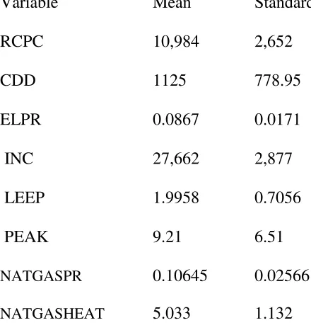
in Table 1; as shown in Table 1, there is no evidence of multicollinearity. Descriptive statistics are provided in Table 2.

In this eclectic model, the greater the total number of cooling degree days in state j in year t (CDDjt), the greater the expected demand for/consumption of residential electricity to cool the interior of residential structures, ceteris paribus (Dodgson, Millward, and Ward, 1990; Sailor and Munoz, 1997; Harris and Liu, 1993; Henley and Peirson, 1998; Yan, 1998; Johnson, 2001; Kamerschen and Porter, 2004; Holtedahl and Joutz, 2004; Moral-Carcedo and Vicens-Otero, 2005; Horowitz, 2007). Interestingly, inclusion of this variable in the analysis is also compatible with the position that cooling a home is one of the two primary sources of demand for residential electricity consumption in the U.S. (National Geographic Society, 2009, p. 84). Following the

“conventional wisdom,” it is expected that the higher the unit price of residential electricity

(ELPRjt), the lower the consumption of same, ceteris paribus (Dodgson, Millward, and Ward, 1990; Harris and Liu, 1993; Holtedahl and Joutz, 2004). As represented in other related studies,

residential electricity is treated as a “normal good” (Dodgson, Millward, and Ward, 1990; Branch, 1993; Harris and Liu, 1993; Holtedahl and Joutz, 2004). Thus, the effect of a higher per capita real personal disposable income (INCjt) on residential electricity consumption is

hypothesized to be positive, ceteris paribus. Natural gas is clearly a substitute for electricity in a variety of household applications, including cooking, hot water production, and home heating. Thus, it is expected that the higher the unit price of natural gas (NATGASPR), the greater the degree of substitution by consumers over time of electricity for natural gas, ceteris paribus

(Dodgson, Millward, and Ward, 1990; Horowitz, 2007). Finally, the variable NATGASHEATjt is a measure of the degree to which natural gas is used rather than electricity to heat residences. The greater the degree to which this usage occurs, the lower the consumption of residential

electricity, ceteris paribus (Dodgson, Millward, and Ward, 1990; Harris and Liu, 1993; Horowitz, 2007).

Based on the initial eclectic model described above, then, it is hypothesized that:

fCDD > 0, fELPR < 0, fINC > 0, fNATGASPR > 0, fNATGASHEAT < 0 (2)

III. Empirical Results

Based on the model expressed in (1) and (2), the following log-log model is to be estimated initially:

log RCPCjt = a0 + a1 log CDDjt + a2 log ELPRjt + a3 log INCjt + a4 log NATGASPRjt

+ a5 log NATGASHEATjt +  (3)

where

a0 = a constant, and

 = a stochastic error term.

(7)

choice of this variable as the instrument was based on the finding that it was highly correlated with ELPRjt while not being correlated with the error terms in the system.

The P2SLS estimation of equation (3), adopting the White (1980) heteroskedasticity correction, is given by:

log RCPCjt = 4.35+ 0.153 log CDDjt – 2.36 log ELPRjt + 0.288 log INCjt (+23.38) (-18.05) (+8.52)

+ 0.363 log NATGASPRjt – 0.048 log NATGASHEATjt, F = 28.15 (4) (+9.03) (-10.83)

where terms in parentheses are t-values.

In estimate (4), all five of the estimated elasticities exhibit the expected signs and are statistically significant at the one percent level. The F-statistic is statistically significant at far beyond the one percent level as well, attesting to the overall strength of the model. Thus, this P2SLS estimate implies that annual per residential customer electricity consumption is an increasing function of the annual number of cooling degree days, real per capita personal disposable income, and the real unit price of natural gas. Furthermore, annual per residential customer electricity consumption is a decreasing function of the real unit price of electricity and the percentage of residences heated by natural gas.

The result for the variable log CDDjt implies that a one percent increase in the annual number of cooling degree days would elicit a 0.153 percent increase in per residential customer electricity consumption. The result for the variable log ELPRjt implies that a one percent increase in the real unit price of electricity would reduce per residential customer electricity consumption by 2.36 percent. As for the variable log INCjt, a one percent increase in real per capita personal disposable income would elevate per residential customer electricity

consumption by 0.288 percent. Regarding the variable log NATGASPRjt, a one percent increase in the real unit price of natural gas would elicit a 0.363 percent increase in the per residential customer consumption of electricity. Finally, the result for the variable log NATGASHEATjt implies that a one percent increase in the percentage of residences heated by natural gas would reduce per residential customer electricity consumption by 0.048 percent.

As shown in equation (5), if the same basic model is estimated in semi-log form by P2SLS, using the White (1980) heteroskedasticity correction and using the one year lag of GSP (GSPjt-1) as the instrument, the results are qualitatively compatible with those in equation (4):

log RCPCjt = 9.62+ 0.000158 CDDjt – 10.94 ELPRjt + 0.000667 INCjt (+29.59) (-21.51) (+10.64)

+ 2.608 NATGASPRjt – 0.000141 NATGASHEATjt, F = 34.29 (5) (+17.08) (-9.78)

In particular, based on the results in equation (5), per residential customer electricity consumption is an increasing function of the annual number of cooling degree days, real per capita personal disposable income, and the real unit price of natural gas, while being a

(8)

natural gas.. These semi-log P2SLS findings are in principle consistent with those in the log-log P2SLS estimate in equation (4), thereby affirming the robustness of the basic model.

IV. Estimations of an Expanded Model

Clearly, the basic model considered above can be expanded. To begin, it would seem potentially very relevant and useful to expand the model so as to investigate, albeit perhaps only on a preliminary basis, the impact on annual per residential customer electricity consumption of the level of state government involvement in the establishment of and perpetuation of energy efficiency programs (Horowitz, 2007). Such a measure is provided by a LEEP score, where the

term “LEEP” stands for Level of Energy Efficiency Programs (DSIRE Solar, 2009). To accomplish this extension, this study adopts this cardinal measure (1, 2, 3) reflecting whether a given state j in year t was weakly (LEEP =1), moderately (LEEP = 2), or strongly (LEEP = 3) engaged in energy efficiency program activities (Horowitz, 2007; DSIRE Solar, 2009). It is

hypothesized that the stronger a state government’s commitment to energy efficiency programs, i.e., the higher the LEEP score, the lower the per residential customer electricity consumption level in the state, ceteris paribus.

Integrating the LEEP score into the basic model in equation (3) and the semi-log version thereof, yields the following:

log RCPCjt = b0 + b1 log CDDjt + b2 log ELPRjt + b3 log INCjt + b4 log NATGASPRjt

+ b5 log NATGASHEATjt + b6 log LEEPjt +’ (6)

log RCPCjt = c0 + c1 CDDjt + c2 ELPRjt + c3 INCjt + c4 NATGASPRjt

+ c5 NATGASHEATjt + c6 LEEPjt + ” (7)

where b0 and c0 are constants, LEEPjt is the cardinal LEEP score for state j in year t, and ’ and

” are error terms.

The P2SLS estimations of equations (6) and (7), adopting the White (1980) heteroskedasticity correction, yield equations (8) and (9), respectively:

Log RCPCjt = 1.49 + 0.124 Log CDDjt – 2.326 Log ELPRjt + 0.502 Log INCjt (+6.71) (-4.27) (+2.73)

+ 0.51 Log NATGASPRjt - 0.068 Log NATGASHEATjt (+3.67) (-4.44)

-0.154 Log LEEPjt, F = 23.43 (8) (-2.41)

Log RCPCjt = 9.79 + 0.000154 CDDjt – 12.42 ELPRjt + 0.00079 INCjt (+28.97) (-131.96) (+6.83)

+ 2.638 NATGASPRjt - 0.00017 NATGASHEATjt (+16.02) (-8.16)

(9)

In estimations (8) and (9) above, all 12 of the estimated elasticities and coefficients exhibit the expected signs; furthermore, 11 are statistically significant at the one percent level and one is statistically significant at the two percent level. Thus, once again, there is strong empirical evidence that annual per residential customer electricity consumption is positively impacted by the annual number of cooling degree days, real per capita personal disposable income, and real natural gas prices, while being negatively impacted by real electricity prices and the percentage of residences heated with natural gas. Furthermore, in both the log-log and semi-log P2SLS estimates, there is compelling evidence that stronger state government involvement in the establishment and perpetuation of energy efficiency programs helps to reduce per residential customer electricity consumption. For example, from equation (8), it appears that a one percent increase in the state commitment to energy efficiency programs reduces per capita residential electricity consumption by 0.154 percent.

Finally, a second extension of the model is introduced. In this extension, an additional factor is controlled for, namely, peak summer electricity production capacity. In particular, we now add the variable PEAKCAPjt, defined, for state j and year t, as “peak summer electricity generation capacity per electricity customer,” (Electrical Power Annual-State Data Table, 2008) to the model in equations (6) and (7), thereby yielding equations (10) and (11), respectively:

log RCPCjt = d0 + d1 log CDDjt + d2 log ELPRjt + d3 log INCjt + d4 log NATGASPRjt

+ d5 log NATGASHEATjt + d6 log LEEPjt + d7 PEAKCAPjt + * (10)

log RCPCjt = e0 + e1 CDDjt + e2 ELPRjt + e3 INCjt + e4 NATGASPRjt

+ e5 NATGASHEATjt + e6 LEEPjt + e7 PEAKCAPjt + ** (11)

This peak capacity in state j in year t (PEAKCAPjt) is determined by the maximum summer electricity output per customer generated in state j in year t by the sources which supply electricity for residential consumption, whether it be generated from a hydro-electric source, a nuclear source, wind, a solar source, coal or any other electricity generating method. The

capacity is denoted as the peak “summer” capacity due to the fact that maximum electricity

consumption traditionally occurs during the peak consumption hours through the hot summer months. Presumably, greater summer generating capacity facilitates greater electricity

consumption (and, indeed, tends to help prevent “brownouts” and “blackouts”), ceteris paribus. Thus, introducing the “supply-side” variable PEAKCAPjt controls for this enhanced ability to use electricity during the summer months.

The P2SLS estimates of equations (10) and (11) are provided by (12) and (13), respectively:

Log RCPCjt = 0.049 + 0.142 Log CDDjt – 2.53 Log ELPRjt + 0.66 Log INCjt (+11.24) (-14.52) (+4.68)

+ 0.52 Log NATGASPRjt - 0.063 Log NATGASHEATjt (+8.69) (-5.89)

(10)

Log RCPCjt = 9.69 + 0.000148 CDDjt – 11.43 ELPRjt + 0.00078 INCjt (+28.17) (-134.22) (+7.27)

+ 2.36 NATGASPRjt - 0.00019 NATGASHEATjt (+13.80) (-11.91)

-0.0339 LEEPjt + 0.0065 PEAKCAPjt, F = 30.91 (13) (-6.30) (+4.85)

Inequations (12) and (13), all 14 of the estimated coefficients exhibit the expected signs, with all 14 being statistically significant at the one percent level. Hence, the results shown in equations (12) and (13) affirm the results provided earlier in this study. Furthermore, they also demonstrate that it may be appropriate to allow for peak summer electricity-producing capacity when investigating determinants of residential electricity consumption. Finally, there is

additional compelling evidence that stronger state government involvement in the establishment and perpetuation of energy efficiency programs helps to reduce per residential customer

electricity consumption. For example, from equation (12), it appears that a one percent increase in the state commitment to energy efficiency programs reduces per capita residential electricity consumption by 0.187 percent.

V. Conclusion

This empirical study provides recent evidence on determinants of annual per residential customer electricity consumption in the U.S. Panel two-stage least squares estimates for the period 2001 through 2005 of both log-log and semi-log specifications consistently provide robust empirical findings. In particular, it is found that annual per residential customer electricity

consumption is an increasing function of the annual number of cooling degree days, real per capita personal disposable income, and the real unit price of natural gas (per cubic foot). Annual per residential customer electricity consumption is also found to be a decreasing function of the real unit price of residential electricity (per kilowatt hour)1 and the percentage of residences heated by natural gas, as well as the degree to which each state has pursued energy efficiency policies. The latter finding provides hope that intelligent public policy can potentially be useful in addressing the environmental challenges presented by residential electricity needs in the 21st century. Lastly, there is evidence that it may be appropriate to allow for peak summer capacity (a

“supply-side” control variable) when investigating determinants of residential electricity consumption.

(11)

Endnote

1_{The finding in this study is that the own price elasticity of the per residential customer demand}

for electricity lies in the range of 2.3 to 2.5 in absolute value terms.

References

ACCRA. 2001. The Council for Community and Economic Research. Fairfax, VA: George Mason University.

American Society of Civil Engineers. 2009. America’s Infrastructure Report Card for 2009. Washington, D.C.: American Society of Civil Engineers.

Bohi, D. R. (1984). Price Elasticities of Demand for Energy: Evaluating the Estimates. Washington, D.C.: Resources for the Future.

Branch, E. R. (1993). “Short-run Income Elasticity of Demand for Residential Electricity Using

Consumer Expenditure Survey Data,” Energy Journal, 14 (1): 111-121.

Dodgson, J. S., Millward, R., and Ward, R. (1990). “The Decline in Residential Electricity

Consumption in England and Wales,” Applied Economics, 22 (1): 59-68.

Dubin, J. A., and McFadden, D. L. (1984). “An Econometric Analysis of Residential Electric Appliance Holdings and Consumption,” Econometrica, 52 (2): 342-362.

DSIRE Solar. (2009). “Incentives for Energy Efficiency,” http://www.dsireusa.org/, Accessed May 28, 2009.

Electric Power Annual-State Data Table. (2008). “Retail Customers by State, Retail Sales of Electricity by State, Average Price by State,”

http://www.eia.doe.gov/cneaf/electricity/epa/epa_sprdshts.html, Accessed May 28, 2009.

Energy Information Administration. (2006). “Annual Energy Outlook, with Projections

to 2030,” http://www.eia.doe.gov/oiaf/archive/aeo06/preface.html, Accessed May 28, 2009.

Garbacz, C. (1983). “A Model of Residential Demand for Electricity Using a National

Household Sample,” Energy Economics, 5 (1): 124-128.

Halstead, J. M., Stevens, T. H., Harper, W., and Hill, B. (2004). “Electricity Deregulation and the Valuation of Visibility Loss in Wilderness Areas: A Research Note,” Journal of Regional Analysis and Policy, 34 (1): 85-95.

Halvorsen, R. (1975). “Residential Demand for Electricity,” Review of Economics and Statistics, 57 (1): 112-18.

Halvorsen, R. (1978). Econometric Models of U.S. Energy Demand. Lexington, MA: Lexington Books.

(12)

Electricity Consumption,” International Journal of Forecasting, 9(4): 437-455.

Henley, A. and Peirson, J. (1998). “Residential Energy Demand and the Interaction of Price

and Temperature: British Experimental Evidence, “ Energy Economics, 20 (2): 157-171.

Holtedahl, P., and Joutz, F. L. (2004). “Residential Electricity Demand in Taiwan,” Energy Economics, 26(2): 201-224.

Horowitz, M. J. (2007). “Changes in Electricity Demand in the United States from the 1970s to

2003,” The Energy Journal, 28(3): 93-119.

International Energy Agency. (2008). World Energy Outlook, 2008. Paris, France: International Energy Agency.

Johnson, T.A. (2001). “Demand, Generation, and Price in the Norwegian Market for Electric

Power,” Energy Economics, 23 (1): 157-171.

Joskow, P.L. (1997). “Restructuring, Competition, and Regulatory Reform in the U.S. Electricity Sector,” Journal of Economic Perspectives, 11 (3): 119-138.

Kamerschen, D. R., and Porter, D. V. (2004). “The Demand for Residential, Industrial and Total Electricity, 1973-1998,” Energy Economics, 26(1): 87-100.

Moral-Carcedo, J., and Vicens-Otero, J.(2005). “Modeling the Non-linear Response of Spanish Electricity Demand to Temperature Variations,” Energy Economics, 27(3): 477-494.

National Climatic Data Center. (2008). “Heating and Cooling Degree Data.” Washington, D.C.,

http://www.ncdc.noaa.gov, Accessed May 28, 2009.

National Geographic Society. (2009). National Geographic. Washington, D.C.: National Geographic Society, June 22.

Natural Gas Demand. (2009). “Short and Long Term Demand for Natural Gas,”

http://www.NaturalGas.org, Accessed May 28, 2009.

Renas, S.M. (1978). “The Cost of Living, Labor Market Opportunities, and the

Migration Decision,” Annals of Regional Science, 15 (1): 95-104.

Renas, S.M. (1983). “The Cost of Living, Labor Market Opportunities, and the

Migration Decision: More on Problems of Misspecification and

Aggregation Bias,” Annals of Regional Science, 17 (1): 98-110.

Sailor, D. J., and Munoz, J. R. (1997). “Sensitivity of Electricity and Natural Gas Consumption to Climate in the U.S.A.: Methodology and Results for Eight States,” Energy, 22 (10): 987-998.

Serow, W.J., Charity, D.A., Fournier, G.M., and Rasmussen, D.W. (1986). “Cost of Living Differentials and Elderly state Migration,” Research on Aging, 8 (2): 317-327.

Taylor, L.D. (1975). “The Demand for Electricity: A Survey,” Bell Journal of Economics, 6 (1): 74-110.

U.S. Census Bureau (2002). Statistical Abstract of the United States, 2002. Washington, D.C.: U.S. Government Printing Office.

(13)

Walden, M.L., and Newmark, C.M. (1995). “Interstate Variation in Teacher Salaries,” Economics of Education Review, 14 (4): 395-402.

White, H. (1980). “A Heteroskedasticity-Consistent Covariance Matrix Estimator and a Direct Test for Heteroskedasticity,” Econometrica, 48 (4): 817-838.

Yan, Y. Y. (1998), “Climate and Residential Electricity Consumption in Hong Kong,” Energy, 23 (1): 17-20.

(14)

Table 1. Correlation Matrix

CDD ELPR INC LEEP PEAKCAP NATGASPR NATGASHEAT

CDD 1.0

ELPR 0.014 1.0

INC -0.089 0.193 1.0

LEEP -0.054 -0.278 -0.045 1.0

PEAKCAP 0.184 -0.304 -0.017 0.128 1.0

NATGASPR 0.427 0.319 0.291 -0.268 0.081 1.0

(15)

[image:15.612.108.328.105.338.2]

Table 2. Descriptive Statistics

Variable Mean Standard Deviation

RCPC 10,984 2,652

CDD 1125 778.95

ELPR 0.0867 0.0171

INC 27,662 2,877

LEEP 1.9958 0.7056

PEAK 9.21 6.51

NATGASPR 0.10645 0.02566