Munich Personal RePEc Archive
Analysing Heterogeneity in Global
Production Technology and TFP: The
Case of Manufacturing
Eberhardt, Markus and Teal, Francis
Centre for the Study of African Economies, Department of
Economics, University of Oxford
19 June 2009
Online at
https://mpra.ub.uni-muenchen.de/15867/
Analysing Heterogeneity in Global
Production Technology and TFP:
The Case of Manufacturing
∗MarkusEberhardt† FrancisTeal
Centre for the Study of African Economies, Department of Economics, University of Oxford
19th June 2009
Abstract:
In this paper we ask how technological differences in manufacturing production across countries can best be modeled when using a standard production function approach. We emphasise the importance of allowing for differences in the impact of observables and unobservables across countries, as well as of data time-series properties. Our novel two-stage estimator, similar to the Pesaran (2006) Common Correlated Effects approach, can account for these matters. Empirical results and diagnostic testing provide strong sup-port for technology heterogeneity. Results are supsup-ported when we adopt an econometric approach allowing for reverse causality. In the light of these findings the interpretation of regression intercepts as TFP levels collapses and we introduce an alternative measure.
Keywords: Manufacturing Production; Parameter Heterogeneity; Nonstationary Panel Econometrics; Common Factor Model; Cross-section Dependence
JEL classification: C23, O14, O47
∗We are grateful to Stephen Bond, Hashem Pesaran and Ron Smith for helpful comments and
sug-gestions. Previous versions of this paper were presented at the Gorman Student Research Workshop and the Productivity Workshop, Department of Economics, University of Oxford (February 2008), at the Nordic Conference for Development Economics in Stockholm (June 2008), at the Economic & Social Research Council (ESRC) Development Economics conference in Brighton (September 2008) and at the International Conference for Factor Structures for Panel and Multivariate Time Series Data in Maastricht (September 2008). All remaining errors are our own. The first author gratefully acknowledges financial support during his doctoral studies from the ESRC, Award PTA-031-2004-00345.
†Corresponding author. Mailing address: Centre for the Study of African Economies, Department
“As a careful reading of Solow (1956, 1970) makes clear, the stylized facts for which this model was developed were not interpreted as universal properties for every country in the world. In contrast, the current literature imposes very strong homogeneity assumptions on the cross-country growth process as each country is assumed to have an identical . . . aggregate production function.”
Durlauf, Kourtellos, and Minkin (2001, p.929)
“In some panel data sets like the Penn-World Table, the time series components have strongly evident nonstationarity, a feature which received virtually no attention in traditional panel regression analysis.”
Phillips and Moon (2000, p.264)
“Most of the work carried out on panel data has usually assumed some form of cross sectional independence to derive the theoretical properties of various inferential procedures. However, such assumptions are often suspect . . . ”
Kapetanios, Pesaran, and Yamagata (2008, p.2)
Why do we observe such dramatic differences in labour productivity across countries in
the macro data? This question has been central to the empirical investigation of growth
and development over the past decades. As the above quotes indicate the importance of
parameter heterogeneity and variable nonstationarity, as well as cross-section dependence,
have not been major concerns in this empirical investigation. In this paper we argue that
all of these issues are important for understanding cross-country differences in labour
pro-ductivity and their causes.
The possibility that technology differences across countries, in the form of parameter
heterogeneity, may be an important part of the growth process has been recognised in both
the theoretical and empirical literature. There is a strand of the ‘new growth’ literature
which argues that production functions differ across countries and seeks to determine the
sources of this heterogeneity (Durlauf et al., 2001). The model by Azariadis and Drazen
(1990) can be seen as the ‘grandfather’ for many of the theoretical attempts to allow for
countries to possess different technologies from each other (and/or at different points in
time).1
The empirical implementation of parameter heterogeneity has primarily occurred
in the empirical convergence literature, with factor parameters initially assumed
group-specific (e.g. Durlauf & Johnson, 1995; Caselli, Esquivel, & Lefort, 1996; Liu & Stengos,
1999) and more recently country-specific (Durlauf et al., 2001).
1Examples of theoretical papers on factor parameter heterogeneity in the production function are
The second feature on which we will focus in the empirical analysis is the time-series
prop-erties of the macro panel data investigated. In the long-run, macro variable series such as
gross output or capital stock often display high levels of persistence, such that it is not
unreasonable to suggest for these series to be nonstationary processes (Nelson & Plosser,
1982; Granger, 1997; Lee, Pesaran, & Smith, 1997; Pedroni, 2007; Canning & Pedroni,
2008). In addition, a number of empirical papers report nonstationary evolvement of
To-tal Factor Productivity (TFP), whether analysed at the economy (Coe & Helpman, 1995;
Kao, Chiang, & Chen, 1999; Bond, Leblebicioglu, & Schiantarelli, 2004) or the sectoral
level (Bernard & Jones, 1996; Funk & Strauss, 2003).
Standard empirical growth studies at the macro level abstract from interdependencies
across countries resulting from common shocks to these economies. In the context of
cross-country growth and development analysis, the potential for this type of data
depen-dency is particularly salient, given the interconnectedness of countries through history,
geography and trade relations. Recent work in the panel time-series literature has aimed
to relax the standard assumption of cross-section independence. This has led to the
devel-opment of analytical methods robust to the impact of correlation across panel units (Bai &
Ng, 2004; Pesaran, 2006, 2007; Kapetanios et al., 2008). Empirical work which allows for
cross-section dependence in panel data is still relatively limited, e.g. production functions
for Italian regions (Costantini & Destefanis, 2009) or Chinese provinces (Fleisher, Li, &
Zhao, 2009).
In this paper we argue that many of the empirical puzzles created in this literature (e.g.
an excessively large capital coefficient) can be resolved once we allow for parameter
hetero-geneity, the nonstationary evolution of most macro data and the role of common factors
in inducing cross-section dependence. Our empirical analysis uses panel data for
manufac-turing from 48 developing and developed countries to show that the technology parameter
estimates differ significantly, depending on whether we do or do not allow for
heterogene-ity and cross-section dependence. Our choice of sectoral data is driven by the notion
when investigating growth and development against the background of structural change
(Temple, 2005; Vollrath, 2009): sectors as diverse as manufacturing, services and
agricul-ture are likely to be characterised by different production technologies, such that separate
estimation is desirable. With regard to our analysis of technology heterogeneity, the
man-ufacturing sector can be argued to be more homogeneous in its production technology
across diverse sets of countries than a representative production technology for the
aggre-gate economy.
The remainder of this study is structured as follows: in the next section we set out a
model which is sufficiently general to encompass the issues raised above. Section two
discusses the empirical implementation of this general framework, presenting a number
of standard and novel estimation strategies. In section three we apply our model to
an unbalanced panel dataset for manufacturing (UNIDO, 2004) to estimate production
functions for 48 countries over the period from 1970 to 2002. Section four discusses formal
parameter heterogeneity tests, while Section five tests the robustness of our findings to
reverse causality. Section six introduces a new methodology for TFP level estimates valid
in the heterogeneous technology case. Section seven concludes.
1
A general empirical framework for production analysis
with cross-country panel data
We adopt a common factor representation for the production function model with
assump-tions as detailed below: fori= 1, . . . , N and t= 1, . . . , T, let
yit = βi′xit+uit uit=αi+λ′ift+εit (1)
xmit = πmi+δ′migmt+ρ1mif1mt+. . .+ρnmifnmt+vmit (2)
where m= 1, . . . , k and f·mt ⊂ ft
whereyit represents gross output or value-added and xit is a vector of observable
factor-inputs including labour, capital stock and in the gross-output specification materials (all
in logarithms).2
For unobserved TFP we employ the combination of a country-specific
TFP levelαi and a set of common factors ft with country-specific factor loadings λi —
TFP is thus in the spirit of a ‘measure of our ignorance’ (Abramowitz, 1956) and
oper-ationalised via an unobserved common factor representation. In equation (2) we further
add an empirical representation of the k observable input variables, which are modelled
as linear functions of unobserved common factors ft and gt, with country-specific factor
loadings respectively. The model setup thus introduces cross-section dependence in the
observables and unobservables. As can be seen, some of the unobserved common factors
driving the variation inyitin equation (1) also drive the regressors in (2). This setup leads
to endogeneity whereby the regressors are correlated with the unobservables of the
pro-duction function equation (uit), making it difficult to identify βi separately from λi and
ρi(Kapetanios et al., 2008). Equation (3) specifies the evolution of the unobserved factors.
We maintain the following assumptions for the empirical model and the data:
A.1 The βi parameters are unknown random coefficients with fixed means and finite
variances. Similarly for the factor loadings, i.e. λi=λ+ηi whereηi ∼iid(0,Ωη).3 A.2 Error terms εit∼ N(0, σ2), whereσ2 is finite. Similarly forvmit and ǫt.
A.3 λ′iftcaptures time-varying unobservables (TFP) and can contain elements which are
common across countries as well as elements which are country-specific.
A.4 The unobserved common factors ftand gmt and therefore the observable inputsxit
and output yit are nota priori assumed to be stationary processes/variables.
A.5 There is an overlap between the unobserved common factors driving output and the
regressors (f·mt ⊂ ft), creating difficulties for the identification of the technology
parameters βi.
2Parameter estimates and interpretation will differ between a value-added based and gross-output based
empirical specification, but if we assume constancy of the material-output ratio we can transform results to make them directly comparable:βiva=βi/(1−γi) (S¨oderbom & Teal, 2004).
3The assumption of random coefficients is for convenience. Based on the findings by Pesaran and Smith
The two most important features of the above setup are the potential nonstationarity
of observables and unobservables (yit,xit,ft,gmt), as well as the potential heterogeneity
in the impact of observables and unobservables on output across countries (αi,βi,λi).
Taken together these properties have important bearings on estimation and inference in
macro panel data which are at the heart of this paper.
2
Empirical implementation
In this Section we first discuss the investigation of variable time-series and cross-section
correlation properties in macro panel datasets. The following subsection then introduces
our novel estimation approach which allows for heterogeneity in the impact of observables
and unobservables, and compares it to the Pesaran (2006) CCE approach.
2.1 Data time-series and cross-section correlation properties
A panel of considerable time-series dimension T opens up the opportunity to use both
country-specific tests from the time-series literature as well as panel-based tests — see
Enders (2004), Hamilton (1994) or Maddala and Kim (1998) for a discussion of the
for-mer, and Choi (2007), Basile, Costantini, and Destefanis (2005) or Smith and Fuertes
(2004, 2007) for a discussion of the latter. Standard time-series unit root tests are
well-known to have low power, such that as the autoregressive parameter approaches unity the
test is less and less able to distinguish between a true unit root (the null hypothesis of the
test) and a false null. “One of the primary reasons behind the application of unit root
tests . . . to a panel of cross-section units was to gain statistical power and to improve on
the poor power of their univariate counterparts” (Breitung & Pesaran, 2005, p.2). Many
panel unit root and cointegration tests discussed in the literature however cannot shake
off an inherent difficulty in terms of interpretation, whereby the null of nonstationarity
(or stationarity or cointegration or noncointegration) forall countries in the panel is
con-trasted with an alternative that at least one country is stationary (or nonstationary or
noncointegrated or cointegrated). Panel unit root test results are often highly sensitive to
across countries or whether information criteria should inform on individual countries’
‘ideal’ lag structure. More recently it was also suggested that correlation across units of
the panel may bias results from ‘first generation’ panel unit root tests (Pesaran, 2007).
Since the seminal contribution by Bai and Ng (2004) the ‘second generation’ literature for
these tests which allows for cross-section dependence has been developing rapidly, with
recent contributions integrating the impact of structural breaks (Westerlund, 2006) and
changes in the volatility of innovations (Hanck, 2008).
In Pedroni (2007) empirical analysis is confined to countries where the data is argued to be
I(1) and cointegrated. In this paper we propose using estimation methods that are robust
to the potential for nonstationarity and cointegration within some, but not all countries
in the panel. This approach is less dependent on making assumptions about the data
which are difficult to test in relatively short panels.4
Further note that unit root evolution
should not be seen as continuing indefinitely (‘global’ property) but represents a ‘local’
behaviour of variableswithin-sample as suggested by Pedroni (2007).
Panel data econometrics over the recent years has seen a rising interest in models with
unobserved time-varying heterogeneity induced by unobserved common shocks that affect
all units (in our present interest: countries), but perhaps to a different degree (Coakley,
Fuertes, & Smith, 2006). This type of heterogeneity introduces cross-section correlation or
dependence between the regression error terms, which can lead to inconsistency and
incor-rect inference in standard panel econometric approaches (Phillips & Sul, 2003; Pesaran,
2006; Pesaran & Tosetti, 2007). The latter typically assume ‘cross-section independence’,
not necessarily because this feature is particularly intuitive given real-world circumstances,
but “in part because of the difficulties characterizing and modelling cross-section
depen-dence” (Phillips & Moon, 1999, p.1092). In the context of cross-country productivity
analysis, the presence of correlation between macro variable series across countries seems
particularly salient.
4Here and in the following we judge the length of a panel with the eyes of a time-series econometrician,
If we assume factorsft (and gmt) in our general model above are stationary, the
consis-tency of standard panel estimators such as a pooled fixed effect regression or a Pesaran
and Smith (1995) Mean Group regression with country-specific intercepts rests on the
pa-rameter values (factor loadings) of the unobserved common factorscontained in both the
y and x-equations: if their averages are jointly non-zero (¯λi 6= 0 and ρ¯i6= 0) a regression
ofy on x and N intercepts (in the pooled fixed effects regression case) will be subject to
the omitted variable problem and hence misspecified, since regression error terms will be
correlated with the regressor, leading to biased estimates and incorrect inference (Coakley
et al., 2006; Pesaran, 2006). In the case of nonstationary factors the consistency issues
in the same framework is altogether more complex and will depend on the exact overall
specification of the model. However, regardless of their order of integration, standard
estimation approaches neglecting common factors will not yield an estimate of β or the
mean ofβi, but ofβi+λiρ−i 1, as shown by Kapetanios et al. (2008) —βi is unidentified. Under the specification described, a standard pooled fixed effects or Pesaran and Smith
(1995) Mean Group estimator will therefore likely yield an inconsistent estimator (due to
residual nonstationarity) of a parameter we are not interested in (due to the identification
problem).
2.2 Empirical estimators
Our empirical approach emphasises the importance of parameter and factor loading
het-erogeneity across countries. The following 2×2 matrix indicates how the various estimators
implemented below account for these matters.5
We abstract from discussing the standard
panel estimators here in great detail and refer to the overview article by Coakley et al.
(2006), as well as the papers by Pedroni (2000, 2001) (GM-FMOLS) and Pesaran (2006)
(CCEP/CCEMG) for more details.
5Abbreviations are as follows: POLS — Pooled OLS, FE — Fixed Effects, FD-OLS — OLS with
vari-ables in first differences, MG — Pesaran and Smith (1995) Mean Group, RCM — Swamy (1970) Random Coefficient Model, GM-FMOLS — Pedroni (2000) Group-Mean Fully Modified OLS, CCEP/CCEMG — Pesaran (2006) Common Correlated Effects estimators, and AMG/ARCM — Augmented MG and RCM, described in detail below. Note that our FE estimator (like the OLS and FD-OLS) is augmented with
Factor loadings:
homogeneous heterogeneous
Technology parameters: homogeneous POLS, FE, FD-OLS CCEP
heterogeneous MG, RCM, GM-FMOLS AMG, ARCM, CCEMG
Essentially, in our model setup all estimators neglecting the heterogeneity in
unobserv-ables (left column) suffer from an identification problem described above. In addition,
the time-series properties of both observable and unobservable processes create further
difficulties for estimation and inference in these empirical approaches: misspecification of
the empirical equation can lead to nonstationary error terms, inducing the breakdown of
any cointegrating relationship in the data.6
Inference is problematic in this case since
conventional standard errors will be invalid, and the associated standard t-statistics will
diverge away from zero with unit probability asymptotically (Kao, 1999). Among the
es-timators neglecting heterogeneity in unobservables the Pedroni (2000) GM-FMOLS is the
only approach to avoid this issue by adopting a nonstationary panel econometric approach
relying on cointegrated variables.
The estimatorsallowing for heterogeneity in factor loadings adopted here (right column)
operate through augmenting the regression equation(s) with ‘proxies’ or estimates for the
unobserved common factors. This augmentation avoids the identification problem and is
also an appropriate strategy to account for cross-section dependence in the presence of
nonstationary variables (Kapetanios et al., 2008). It is in this context that we introduce
our own estimators, namely the Augmented Mean Group (AMG) and Swamy Random
Coefficient Model (ARCM) estimators which are the focus of the following discussion.
The Augmented Mean Group (AMG) estimator accounts for cross-section dependence
by inclusion of a ‘common dynamic process’ in the country regression. This process is
6As developed by Phillips and Moon (1999, p.1091) estimation equations which result in nonstationary
extracted from the year dummy coefficients of a pooled regression in first differences
(FD-OLS) and represents the levels-equivalent mean evolution of unobserved common factors
across all countries. Provided the unobserved common factors form part of the
country-specific cointegrating relation (Pedroni, 2007), the augmented country regression model
en-compasses the cointegrating relationship, which is allowed to differ across countries:
Stage (i) ∆yit =b′∆xit+ T X
t=2
ct∆Dt+eit ⇒cˆt≡µˆ•t (4)
Stage (ii) yit=ai+b′ixit+cit+diµˆ•t+eit ˆbAM G=N−
1X
i
ˆbi (5)
The first stage represents a standard FD-OLS regression withT−1 year dummies in first
differences,7
from which we collect the year dummy coefficients which are relabelled as
ˆ µ•
t. This process is extracted from the pooled regression in first differences since
non-stationary variables and unobservables are believed to bias the estimates in the pooled
levels regressions. There is also some evidence (Monte Carlo results available on request)
that the identification problem forβi we discussed earlier is addressed successfully in the
FD-OLS approach. FD-OLS yields an estimate of the common technology parameters or
an unweighted mean of the country-specific cointegrating coefficients (Smith & Fuertes,
2007), depending on the assumptions about the underlying technology parametersβi. The
underlying common factors (in the levels equation) can be stationary or nonstationary.
In the second stage this estimate ˆµ•
t is included in each of the N standard country
re-gressions which also include linear trend terms to capture omitted idiosyncratic processes
evolving in a linear fashion over time. Alternatively we can subtract ˆµ•
t from the
depen-dent variable, which implies the common process is imposed on each country with unit
coefficient (not shown).8
In either case the AMG estimates are then derived as averages of
the individual country estimates, following the Pesaran and Smith (1995) MG approach.
Based on the results of Monte Carlo simulations (available on request) we posit that the
7Year dummies in first differences result in alevels seriesfor the unobserved average/common factors,
rather than the annual growth rates as would be the case for levels year dummies in a model where inputs and output are in first differences.
8Note further that unity is also the cross-country average parameter expected for the coefficients on ˆµ•
t:
¯
d=N−1P
inclusion of ˆµ•
t allows for theseparateidentification ofβi orE[βi] and the unobserved com-mon factors driving output and inputs, like in the Pesaran (2006) CCE case. In analogy to
applying ˆµ•
t in the country equations in levels, we can use ∆ˆµ•t in the country equations in
first differences. Similarly we can augment the Swamy (1970) RCM estimator in a similar
fashion to yield the Augmented Random Coefficient Model (ARCM) estimators in levels
and first differences.
The focus of the CCE estimators is the estimation of consistent ˆband not the nature of the
unobserved common factors or their factor loadings: we cannot obtain an explicit estimate
for the unobserved factors ft or the factor loadings λi, since the average impact of the
factors (¯λ) is unknown. Our augmented estimators use an explicit rather than implicit
estimate forft from the pooled first stage regression in first differences. Compared with
the CCE approach we can obtain an economically meaningful construct from the AMG
setup: the common dynamic process ˆµ•
t =h(¯λft) represents common TFP evolution over
time, whereby common is defined either in the literal sense, or as the sample mean of
country-specific TFP evolution. The country-specific coefficient on the common dynamic
process, ˆdifrom equation (5), represents the implicit factor loading on common TFP.
3
Data and main empirical results
3.1 Data
For our empirical analysis we concentrate on aggregate sectoral data for manufacturing
from developed and developing countries for 1970 to 2002 (UNIDO, 2004). Our sample
represents an unbalanced panel of 48 countries with an average of 24 time-series
obser-vations (1,162 obserobser-vations in levels, 1,094 in first difference regressions — gross output
based sample; for the value-added based sample we have slightly more observations, 1,194
and 1,128 for levels and first difference regressions respectively). For a detailed discussion
and descriptive statistics see Appendix A. Note thatall of the results presented are
strik-ingly robust to the use of a reduced sample constructed with application of a set of rigid
3.2 Time-series properties of the data
We carry out a range of stationarity and nonstationarity tests for individual country
time-series as well as the panel as a whole, results for which are presented in Appendix B.9
The
tests conducted include country-specific unit root tests and panel unit root tests of the first
and second generation. In case of the present data dimensions and characteristics, and
given all the problems and caveats of individual country unit root tests as well as panel
unit root tests, we can suggest most conservatively that nonstationarity cannot be ruled
out in this dataset. Investigation of the time-series properties of the data was not intended
to select a subset of countries which we can be reasonably certain display nonstationary
variable series as in Pedroni (2007); instead, our aim was to indicate that the sample
(possibly due to the limited time-series dimension) is likely to be made up of a mixture of
some countries with stationary and others with nonstationary variables.
3.3 Pooled regressions
We estimate pooled models with variables in levels or first differences, includingT−1 year
dummies or country-specific period-averages `ala Pesaran (2006) to account for unobserved
common factors. In all pooled regressions the slope coefficients on the factor-inputs and
the year dummies are restricted to bethe sameacross all countries. Our results presented
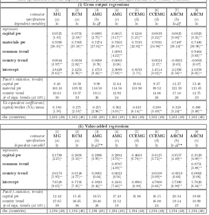
in Tables 1 and 2, in each case for a gross output and value-added specification in the upper
and lower panels respectively, are for the following estimators: for the data in levels we
apply[1]the pooled OLS estimator (POLS); [2]the pooled fixed effects estimator (FE);
[3]the Pesaran (2006) common correlated effects estimator in its pooled version (CCEP);
and [4] the pooled OLS estimator for data in first differences (FD-OLS) — additional
information is contained in the notes to the table. Estimation equations in columns [1],
[2], and [4] of both tables include sets of (T −1) year dummies.
[Table 1 about here]
We first discuss the results for the empirical specification without any restrictions on the
returns to scale — Table 1. Estimates for the factor input parameters in all regressions are
statistically significant at the 5% level or 1% level. The POLS results in column [1]
sug-gest that failure to account for time-invariant heterogeneity across countries (fixed effects)
yields severely biased results: the VA-equivalent capital coefficient from the gross-output
specification in the upper panel at .9 is considerably inflated, with the capital coefficient
from the VA specification in the lower panel somewhat more moderate at .8. Inclusion of
country intercepts in [2] reduces these coefficient estimates somewhat. The same
param-eter in the CCEP results in [3] is yet lower still, around .6. In both the FE and CCEP
estimators the fixed effects are highly significant (F-tests are reported in Table footnote).
For all three estimators in levels the regression diagnostics suggest serial correlation in the
error terms, while constant returns to scale are rejected at the 1% level of significance in
all cases except POLS in the value-added specification. Note that for the FE estimator
the data rejects CRS in favour of increasing returns — an unusual finding. The OLS
regressions in first differences in [4] yields somewhat different technology estimates: the
capital coefficient is now around .3 in both specifications (VA-equivalent), thus in line
with observed macro data on factor share in income (Mankiw, Romer, & Weil, 1992).
CRS cannot be rejected, the AR(1) tests show serial correlation for this model, which is
to be expected given that errors are now in first differences. There is however evidence
of some higher order autocorrelation, especially in the VA-specification. Note that we
obtain identical results for models in [1], [2] and [4] if we use data in deviation from the
cross-sectional mean (results not presented) instead of using a set of year dummies.
Re-placing year dummies with cross-sectionally demeaned data is only valid if parameters are
homogeneous across countries (Pedroni, 1999, 2000) — in the pooled regressions we force
this homogeneity onto the data, such that identical results are to be expected.
Under intercept and technology parameter heterogeneity, given nonstationarity in (some
of) the country variable series the pooled FE estimates in column [3] asypmtotically
con-verge to the ‘long-run average’ relation at speed √N (Phillips & Moon, 1999) provided
T /N → 0 (joint asymptotics) and cross-section independence. In the present sample,
however, nonstationary error terms and unobserved common factors seem to influence the
than twice the magnitude of the macro data on factor shares in income (Mankiw et al.,
1992; Gomme & Rupert, 2004), a common finding in the literature (Islam, 2003; Pedroni,
2007). Further recall thatt-values are invalid for the estimations in levels if error terms
are nonstationary (Coakley, Fuertes, & Smith, 2001; Kao, 1999). The CCEP
estima-tor accounts for cross-section dependence and yields, as the residual analysis in Section
3.6 below suggests, stationary errors terms. The difference estimator in [4] converges to
the common cointegrating vector β or the mean of the individual country cointegrating
relations, E(βi), at speed √T N (Smith & Fuertes, 2007). Further investigation
regard-ing alternative specification with parameter heterogeneity (CCEMG estimator) as well as
residual diagnostics will be necessary to judge the bias of the present CCEP results.
As the model in first differences does not reject constant returns to scale (CRS), we impose
CRS on all models and investigate the outcome — given that we are analysing a ‘global’
production function, the assumption of constant returns should be far from controversial
and may help the data to differentiate between capital and material inputs more readily
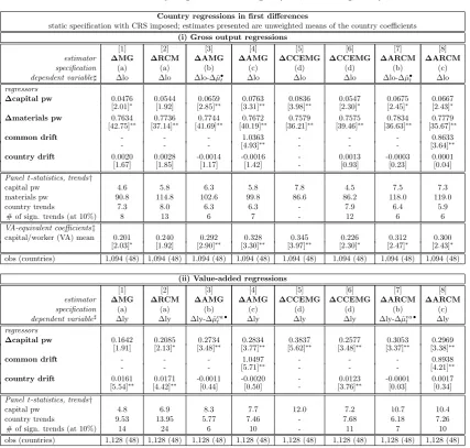
than is evidenced in the previous results. Table 2 presents the results for the pooled
regression models with CRS imposed.
[Table 2 about here]
The imposition of CRS does not alter the pooled regression results in levels to a great
ex-tent: POLS in [1], FE in [2] and CCEP in [3] yield capital coefficient estimates of around
.9, .7 and .6 respectively; in the gross output specification our preferred ∆OLS
estima-tor in [4] now has a slightly less precisely identified capital coefficient, which is however
within the 95% confidence intervals of the estimate in the unrestricted equation.10
The
VA-equivalent capital coefficient as a result has dropped to around .23. In the value-added
specification, the ∆OLS estimates show very similar results for the unrestricted and
re-stricted returns to scale models.
10We also carry out a Wald test for parameter equality and cannot reject the null that they are the
Our pooled regression analysis suggests that time-series properties of the data play an
important role in estimation: the pooled OLS and FE levels regressions, where some or
all country variable series may be I(1), yield very high parameter coefficients on capital,
which translate into VA-equivalent capital coefficients of between .6 to .9. We suggest
that the bias is the result of nonstationary errors, which are introduced into the pooled
equation by the imposition of parameter homogeneity on heterogeneous country equations
— we investigate both matters in more detail below. In contrast, the OLS regressions
where variables are in first differences and thus stationary (FD-OLS) yielded more sensible
capital parameters. This pattern of results fits the case of level-series being integrated of
order one in at least some of the countries in our sample. The results for the CCEP are
somewhat surprising, given our findings when we relax parameter homogeneity.
3.4 Common TFP
Following our argument above, the FD-OLS regression represents the only pooled
re-gression model which estimates a cross-country average relationshipsafe from difficulties
introduced by nonstationarity. We therefore make use of the year dummy coefficients
de-rived from our preferred pooled regressions with CRS imposed (FD-OLS, column [4] in
Table 2) to obtain an estimate of the common dynamic process ˆµ•
t, which represents an
estimate of the common TFP evolvement (mean of the unobserved common factors
eval-uated at the average impact across countries). Figure 1 illustrates the evolvement path of
this common dynamic process for the gross-output based model.11
[Figure 1 about here]
The graph shows severe slumps following the two oil shocks in the 1970s, while the 1980s
and 1990s indicate considerable upward movement.12
The version of this graph for results
from the VA-specification shows the same patterns over time (not reported). Recall that
we favour the ‘measure of ignorance’ interpretation of TFP, such that a decline in global
11In the graph we omit the data-point for 2002 for which there are only two observations. This implied
‘globally common evolution’ is for a gross-output specification. In order to provide a graph translated into a VA specification, we first need to scale the year dummy coefficients by 1/(1−γˆ) to account for material inputs. The resulting TFP evolution (not presented) is very similar to that for the VA specification.
12Note that these graphs are ‘data-specific’: for years where data coverage is good, this can be interpreted
manufacturing TFP as evidenced in the 1970s should not be interpreted as a decline in
knowledge, but a worsening of the global manufacturingenvironment. A simpler
explana-tion may be that our variable deflaexplana-tion13
does not adequately capture all the price changes
in general, and material input price changes vis-`a-vis output prices in particular, occurring
in the post-oil shock periods.
3.5 Country regressions
In the following we relax the assumption implicit in the pooled regressions that all countries
possess the same production technology, and allow for country-specific slope coefficients on
factor inputs. At the same time, we maintain that common shocks and/or cross-sectional
dependence have to be accounted for in some fashion. We contrast models that allow for
unobserved common factors in different ways, with models which ignore these matters. A
total of four specifications are investigated:
(a) yit=ai+bi′xit+cit+eit (6)
(b) yit−µˆ•t =ai+b′ixit+cit+eit (7)
(c) yit=ai+b′ixit+cit+diµˆ•t +eit (8)
(d) yit=ai+b′ixit+d′1iy¯t+d′2ix¯t {+cit}+eit (9)
In specification(a) we do not account for any cross-section dependence and/or common
TFP — this represents standard country regressions augmented with linear country-trends
(trend coefficient ci. Our novel augmented estimator has two variants: in (b) the
com-mon dynamic process ˆµ•
t is imposed with a unit coefficient, whereas in (c) it is included
as additional regressor. The augmentation with cross-section averages is represented by
option(d).
These four specifications are implemented as follows: [1]the standard Pesaran and Smith
(1995) Mean Group (MG) and[2] the Swamy (1970) Random Coefficient Model (RCM)
13Country deflators for monetary values in local currency units [LCU], which are subsequently translated
estimators are representatives of option (a); the Augmented Mean Group (AMG) estimator
can either[3]have the common dynamic process (ˆµ•
t) imposed with unit coefficient like in
option (b), or[4]have it included as additional regressor like in option (c). Similarly for the
Augmented RCM (ARCM)[7],[8]. The Mean Group version of the Common Correlated
Effects estimator (CCEMG) represents option (d). We test two alternative specifications,
namely[5]as defined by Pesaran (2006), and [6]augmented with a country-specific linear
trend term.14
Unweighted averages of country parameter estimates are presented for regressions in
lev-els and first differences in Tables 3 and 4 respectively, with gross-output modlev-els in the
upper panel and value-added models in the lower panel of each table. In all cases we
have imposed constant returns to scale on the country regression equation, in line with
the findings from our preferred pooled model in first differences — this decision and its
implications are discussed in more detail below.
The concept of ‘mean-group’ estimates — be they from MG, CCEMG or the weighted
variant of the Swamy RCM — suggests that whileindividual country regression estimates
may be unreliable, by averaging across the estimates we obtain a more reliable measure of
the average relationship across groups/countries (Pesaran & Smith, 1995). Thet-statistics
for the country-regression averages reported in all tables for country regression results are
measures of dispersion for the sample of country-specific estimates.15
We further provide
the Pedroni (1999) ‘panelt-statistic’ (1/√N)Piti, constructed from the country-specific
t-statistics (ti) of the parameter estimates, which indicates the precision of the individual
country estimates for capital, materials and country-specific linear trend terms. From our
results we can see that the individual country estimates for thelevels specification are on
average more precisely estimated than those in the specifications infirst differences. This
pattern is repeated in the results for the value-added regressions.
14In the first instance we deliberately do not use ‘demeaned’ data, since cross-sectional demeaning is
only valid if all model parameters are homogeneous across countries, but creates bias in case of parameter heterogeneity (Pedroni, 2000; Smith & Fuertes, 2007). We briefly discuss the results for ‘demeaned’ data at the end of this section, referring to Table C-1 in Appendix D.
15In case of the MG-type estimators these are computed from the standard errorsse( ˆβ
M G) = [Pi( ˆβi− ˆ
[Tables 3 and 4 about here]
We begin our discussion with the averaged estimates in the levels specification in Table 3.
Our first observation regarding these results is that acrossall specifications the means of
the capital coefficients are considerably lower than in the pooled levels models: between
.2 and .5 (VA-equivalent) rather than between .6 and .9 in the pooled levels models in
Table 2. Comparing results for the levels specification with those for the specification in
first differences in Table 4 reveals that estimates from the heterogeneous models in levels
and first differences follow very similar patterns. Recall that for the pooled models
esti-mates for technology parameters in levels and first differences showed radically different
results. Parameter estimates are thus similar in all specifications, gross-output or
value-added, levels or first-differences.
In all cases it seems that the technology parameters are estimated reasonably precisely,
suggested by the reportedt-statistic and the Pedroni (1999) panel t-test. A considerable
number of country trends/drifts are significant at the 10% level, although much more so for
the levels than for the first difference specifications — the statistically insignificantmean
in all of the ‘augmented’ regressions (AMG, ARCM) is easily explained: these
country-specific trends have positive and negative magnitudes for different countries. Coefficients
on the common dynamic process ˆµ•
t in models [4] and [8] for all specifications are uniformly
high and close to their theoretical value of unity.
Closer inspection of the VA-equivalent capital coefficients suggests the following patterns:
firstly, estimation approaches that do not account for unobserved common factors or
cross-section dependence have parameter estimates around .2. Secondly, for the ‘augmented’
estimators which include a common dynamic process in the estimation equation (either
explicitly or implicitly with unit coefficient) the capital coefficients are around .3. Thirdly,
the results for the CCEMG with and without additional country trend differ considerably,
with the former close to all other augmented regression results and the latter slightly
In Figures D-1 and D-2 in Appendix D we plot the density estimates for the sample of
country-specific technology parameters estimated in the levels regressions presented in
Table 3, using standard kernel methods with automatic bandwidth selection. Both sets
of plots indicate that the distribution of these parameter estimates is fairly symmetric
around their respective means, such that no significant outliers drive our results.
We also briefly review the results for country regressions where the data was first
trans-formed into deviations from the cross-sectional mean to account for any common dynamic
processes. As was noted previously, this transformation is only valid if the parameters are
homogeneous across countries (Pedroni, 2000). The averaged results for this exercise are
presented in Table C-1 in Appendix C. Here, the gross output specifications (levels, FD)
yield capital coefficients of between .44 and .48 (VA-equivalent). In stark contrast, the
value-added specifications yield capital coefficients between .13 and .20. We take these
results as an indication of technology parameter heterogeneity in the production
func-tion, since as was discussed above the transformation of variables into deviations from the
cross-section mean introduces nonstationarity into the errors if the underlying production
technology differs across countries.
3.6 Residual diagnostics
The nature of our data prevents us from implementing a number of specification tests
from the nonstationary panel econometric literature: first of all, existing procedures used
to investigate cross-section dependence (PCA, mean absolute correlation, Pesaran (2004)
CD statistic for residual diagnostics) rely on fairly balanced panels without missing
ob-servations. Secondly, panel cointegration tests which allow for cross-section dependence
(Westerlund & Edgerton, 2008) perform poorly in moderate T panels, while first
gener-ation test routines are developed with balanced panels of full time-series in mind. It is
unclear how these can be implemented for a macro panel which includes data from
devel-oping countries and thus missing observations and considerable unbalance. We therefore
need to resort to a mix of diagnostic tests for pooled regressions and averaged test statistics
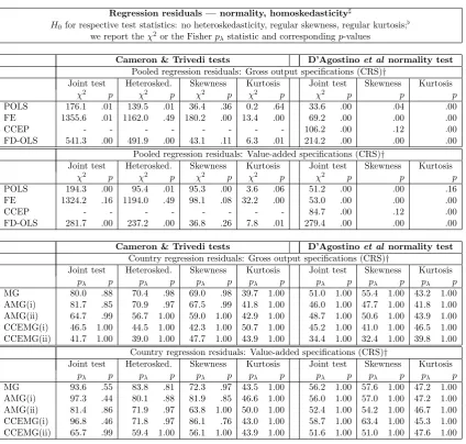
We begin with normality and homoskedasticity tests for regression residuals in Table 5.
Using the D’Agostino, Balanger, and D’Agostino Jr. (1990) and Cameron and Trivedi
(1990) tests virtually all of our pooled regression results reject the joint null hypothesis
of normal, and normal and homoskedastic residuals respectively. In contrast the country
regression residuals can be assumed as jointly normal or jointly normal and homoskedastic,
based on the Fisher statistics (pλ) constructed from these two testing procedures.
[Table 5 about here]
Tables 6 and 7 present panel unit root test results for pooled regression and country
regression errors respectively. This analysis broadly suggests that residuals from from
POLS and FE are likely to be nonstationary. Country regression residuals are more likely
to be stationary across all specifications: nonstationarity is rejected for up to 4 lags in
the first generation Maddala and Wu (1999) test, and still for up to 3 lags in the Pesaran
(2007) CIPS test (CIPS∗), where residuals are not ‘demeaned’ prior to testing.
[Tables 6 and 7 about here]
A cautious conclusion from these diagnostic tests would be that we are more confident
about the country regression residuals possessing desirable properties (stationarity,
nor-mality, homoskedasticity) than we are for their pooled counterparts.
3.7 The importance of constant returns to scale
Further investigation reveals that the imposition of constant returns to scale, justified by
the CRS test for the pooled regression with variables in first differences, plays an
impor-tant role in our story. We repeat all country regressions in levels, but with all variables
‘levels’ form, rather than in per worker terms. Results are presented in Table C-2 below.
The failure to impose constant returns to scale leads to a loss of precision in the capital
es-timates in virtually all specifications, for the regressions in levels and first differences. The
labour coefficients are however around .7 in all cases and only one out of 16 levels models
rejects a parameter test for constant returns to scale — the latter result is not surprising
given the sizeable standard errors on the capital coefficients. In the first difference models
difference between the impact of imposing CRS in the country regressions (considerable
loss of precision) and the pooled regressions (limited change) is somewhat puzzling and
merits further investigation in the future.
3.8 Discussion of main empirical results
Our analysis investigated the changing parameter estimates across a number of empirical
specifications and estimators. Our pooled estimators in levels are suggested to be severely
biased, given the diagnostic tests and the fact that their capital coefficients range from
.6 to .8 (VA-equivalent), far in excess of the macro evidence of around 1/3. There may
be a number of possible sources for this bias: firstly, if parameter heterogeneity prevails
and variable series are indeed nonstationary the imposition of common technology across
countries leads to nonstationary errors and thus noncointegration. Secondly, the results
may be the outcome of an identification problem, which arises if the same unobserved
common factors drive both output and inputs. In this case the pooled estimates (with the
exception of the CCEP) cannot identify the technology parametersβ separately from the
impact of unobserved factorsλi. The fact that CCEP yields very similar results to POLS
and FE suggests that interplay of parameter heterogeneity and variable stationarity plays
an important role.
The first difference estimator (FD-OLS) in contrast has rather sound diagnostics and yields
sensible parameter coefficients. The empirical properties of this estimator are somewhat
unclear, especially with regard to the identification issue.
The heterogeneous parameter estimators uniformly yield lower implied capital coefficients
more in line with the aggregate economy factor income share data. Across levels and
first difference, gross-output and value-added specifications there seems to be a consistent
pattern emerging whereby the standard heterogeneous estimators (MG, RCM) obtain
qual-itatively different results from the augmented heterogeneous estimators (AMG, ARCM,
however we can argue that the MG and RCM estimators are likely to be biased for two
rea-sons: firstly, they use an overly simplified representation for TFP evolution (linear trend)
which requires stationarity. Secondly, as was discussed above, these estimators are argued
to suffer from an identification problem whereby the technology parametersβi cannot be
identified separately from the impact of unobserved common factors on outputλi in the
case where the same unobserved common factors drive output and inputs (Kapetanios et
al., 2008).
Turning to the augmented estimators, we suggest that the combination of a common
dy-namic process and a linear country trend is confirmed by the data: a considerable number
of country trends are statistically significant, while the cross-country average coefficient for
ˆ µ•
t is close to unity in the model where it is included as additional regressor. The CCEMG
estimator provides results broadly in line with those for the AMG and ARCM, with the
latter two on the whole more consistent across specifications. The comparison between
the country regression results presented above and the results for ‘demeaned’ variables
in the Appendix indicate that the unobserved common factors exert differential impact
across countries, thus meriting the adoption of approaches which allow for heterogeneous
factor loadings (and thus TFP).
The estimate for globally common or mean TFP evolution ˆµ•
t shows serious dips following
the two oil crisis shocks in 1973 and 1979, with almost continuous growth thereafter from
the mid-1980s to the late 1990s — this development path is arguably in line with historical
events and anecdotal evidence regarding the global evolution of manufacturing over the
thirty-three-year sample period.
As a further robustness test we also carry out pooled and country regressions adopting
a dynamic empirical specification — results do not change considerably in comparison to
4
Testing parameter heterogeneity
The individual country coefficients emerging from the regressions in the previous section
imply considerable parameter heterogeneity across countries. This apparent heterogeneity
may however be due to sampling variation and the relatively limited number of time-series
observations in each country individually (Pedroni, 2007). We therefore carried out a
num-ber of formal parameter heterogeneity tests for the results from the AMG, ARCM and
CCEMG estimations in levels and first difference: firstly, we constructed predicted
val-ues based on the mean parameter estimates of our heterogeneous parameter models, and
regressed these on input variables, a common trend and country intercepts in a pooled
regression. The rationale of this test is that if parameter estimates were truly
hetero-geneous we would not expect significant coefficients on the input variables. Secondly, we
obtained Swamy (1970) ˆSstatistics for levels and first difference specifications. Thirdly, we
constructed Wald statistics following Canning and Pedroni (2008), and fourthly, we
pro-ducedF-statistics for standard and augmented MG estimators following Pedroni (2007).16
Taken together the results for these various tests (available on request) do give a strong
indication that parameter homogeneity is rejected in this dataset. Systematic differences
in the test statistics for levels and first difference specifications indicate that
nonstation-arity may drive some of these results. Nevertheless, even if heterogeneity were not very
significant in qualitative terms, our contrasting of pooled and country regression results
has shown that it nevertheless matters greatly for correct empirical analysis in the presence
of nonstationary variables.
5
Reverse causality
In the analysis of empirical production functions the issue of variable endogeneity is
typ-ically of great concern, requiring means and ways to instrument for factor inputs. A
popular approach to address this problem is to convert macro-panel data into a short
16Further tests for parameter heterogeneity (Phillips & Sul, 2003; Pesaran, Smith, & Yamagata, 2008)
panel of typically 5-year averages and to employ empirical estimators originally developed
for largeN, small T micro-panels (Arellano & Bond, 1991; Blundell & Bond, 1998), e.g.
Islam (1995) and Caselli et al. (1996) for Penn World Table data. For analysis of other
macroeconomic relationships it is also not uncommon to see these estimators used for
annual data whereT becomes moderate to large, despite the difficulties arising from
over-fitting (Bowsher, 2002; Roodman, 2009). When model parameters differ across countries
the instrumentation strategy in these GMM-type estimators (and any other IV strategies
forpooled regressions) however breaks down since informative instruments are invalid by
construction (Pesaran & Smith, 1995). In the following we therefore adopt the
empiri-cal approach by Pedroni (2000, 2007) and estimate country regressions by Fully-Modified
OLS, whereupon parameter estimates are averaged across countries (Group-Mean
FM-OLS). Provided the variables are nonstationaryand cointegrated the individual FMOLS
estimates are super-consistent.
[Table 8 about here]
In the upper panel of Table 8 we present averaged parameter estimates for the full sample
value-added-based FMOLS regressions, where column[1]represents the standard
Group-Mean FMOLS, and columns[2] and [3]augment the country FMOLS equation with the
common dynamic process ˆµ•t,va. Columns[4]and[5]apply FMOLS to a country regression
with the CCE-augmentation before averaging the parameter estimates. In the lower panel
of the same table our sample only includes 26 countries which ‘pass’ two nonstationarity
test (KPSS, ADF) for value-added per worker and capital stock per worker respectively.
Due to the unbalanced nature of our panel we are prevented from testing for cointegration
between these two variables.
The standard Pedroni (2000) approach yields insignificant capital estimates, whereas
aug-mentation with the common dynamic process yields statistically significant estimates very
close to those arising from our previous AMG regressions. Once we include ˆµ•t,va we thus
obtain the same empirical results in the Group-Mean Fully-Modified OLS and Mean Group
OLS approaches. Similar to the results in Table 3 the CCE-augmented average estimate
estimate for capital of around .3.
These results are robust to a restriction of the sample to countries for which value-added
and capital stock per worker ‘pass’ the nonstationarity tests: for the Pedroni (2000)
esti-mator capital stock is insignficant, whereas the inclusion of the common dynamic process
replicates our earlier findings. We take these results as a vindication that the
produc-tion process represents a three-way cointegraproduc-tion between output, factor-inputs and some
unobserved common factors.
6
Estimating TFP in a heterogeneous parameter world
In most applications in the literature the estimation of production functions is just the
first step in an empirical analysis that concentrates on the magnitudes and determinants
of Total Factor Productivity (TFP). In our analysis we have thus far focused on the factor
parameter estimates and their magnitudes and robustness across specifications. We do
however also want to provide some estimates for TFP and its evolution. From the country
regressions we can obtain estimates for the intercept, technology parameters, idiosyncratic
and common trend coefficients or the parameters on the cross-section averages for AMG
and CCEMG specification respectively. One could be tempted to view the coefficients
on the intercepts as TFP level estimates, just like in the pooled fixed effects case.
How-ever, once we allow for heterogeneity in the slope coefficients, the interpretation of the
intercept as estimate for base-year TFP level is no longer valid. Consider the example in
Figure 2.
[Figure 2 about here]
We provide scatter plots for ‘adjusted’ log value-added per worker (y-axis) against log
capital per worker (x-axis) as well as a fitted regression line for these observations in each
of the following four countries: in the left panel France (circles) and Belgium (triangles),
in the right panel South Korea (circles) and Malaysia (triangles). The ‘adjustment’ is
specification (c) and constructed in the following steps:17
we begin with the fitted values
of this estimation
ˆ
yit= ˆai+ ˆbilog(K/L)it+ ˆcit+ ˆdiµˆ•t (10)
where ˆai, ˆbi, ˆci and ˆdi are country-specific estimates for the intercept, log capital per
worker, the common dynamic process and a linear trend term. In order to illustrate our
case, we want to obtain a simple linear relationship between value-added and capital where
the contribution of TFP growth has already been accounted for. We compute
yadjit =yit−cˆit−dˆiµˆ•t (11)
We then plot this variable against log capital per worker for each country separately.
This procedure in essence provides a two-dimensional visual equivalent of the estimates
for the capital coefficient (slope) and the TFP level (intercept) in the augmented country
regression. The left panel of Figure 2 shows two countries (France, Belgium) with
vir-tually identical capital coefficient estimates (slopes). The in-sample fitted regression line
is plotted as a solid line, the out-of-sample extrapolation toward the y-axis is plotted in
dashes. The country-estimates for the intercepts can be interpreted as TFP levels, since
these countries have very similar capital coefficient estimates (ˆbi ≈ˆbj). In this case, the
graph represents the linear modelyitadj = ˆai+ ˆblog(K/L)it, where ˆai possesses the ceteris
paribus property. In contrast, the right panel shows two countries which exhibit very
different capital coefficient estimates (slopes). In this case ˆai cannot be interpreted as
possessing the ceteris paribus quality since ˆbi 6= ˆb: ceteris non paribus! In the graph we
can see that Malaysia has a considerably higher intercept term than South Korea, even
though the latter’s observations lie above those of the former at any given point in time.
This illustrates that once technology parameters in the production function differ across
countries the regression intercept can no longer be interpreted as a TFP-level estimate.
We now want to suggest an alternative measure for TFP-level which is robust to parameter
heterogeneity. Referring back to the scatter plots in Figure 2, we marked the base-year
level of log capital per worker by vertical lines for each of the four countries. We suggest to
use the locus where the solid (in-sample) regression line hits the vertical base-year capital
stock level as an indicator of TFP-level in the base year. In the value-added specification
theseadjusted base-year and final-year TFP-levels are thus
ˆ
ai+ ˆbilog(K/L)0,i and ˆai+ ˆbilog(K/L)0,i+ ˆciτ+ ˆdiµˆ
•
τ (12)
respectively, where log(K/L)0,i is the country-specific base-year value for capital per
worker (in logs), τ is the total period for which country i is in the sample and ˆµ•
τ is
the accumulatedcommon TFP growth for this period τ with the country-specific
param-eter ˆdi. It is easy to see that the intercept-problem discussed above only has bearings on
TFP-level estimates. A similar formula applies for the CCEMG estimator.18
Focusing exclusively on the TFP-levels in the base-year, Table C-3 in Appendix D presents
the rank (by magnitude) for adjusted TFP levels derived from the AMG estimator in
specification (c), i.e. with ˆµ•t included as additional regressor, and the standard CCEMG
estimator (in specification (d)). We further show the country ranking based on a pooled
fixed effects estimation, such as that presented in Table 3, column [2]. As can be seen in
the right half of the table, the rankings differ considerably between the AMG or CCEMG
results on the one hand and standard fixed effects results on the other (median absolute
rank difference (MARD): 10, respectively), but not between the results for AMG and
CCEMG (MARD: 1).
We present adjusted TFP base-year and final-year levels for these AMG and CCEMG
models in Figure D-3 in Appendix D. Note that in our sample base- and final-year differ
across countries (see Table A-2 in Appendix A). The countries in both charts are arranged
in order of magnitude of their final-year adjusted TFP levels in the AMG(ii) model, for
which results are shown in the left bar-chart. With exception of a small number of countries
(e.g. MLT — Malta, SGP — Singapore) the general ordering of countries by final-year
18This adjustment is somewhat more complex, involving the base-year values of cross-section averages
and country-specific coefficients on these averages instead of ˆµ•
TFP levels is very similar in the two specifications: countries such as Finland, Canada,
the United States or Ireland can be found toward the top of the ranking, with Bangladesh,
India, Sri Lanka and Poland closer to the bottom.
7
Overview and conclusions
In this paper we have investigated how technology differences in manufacturing across
countries should be modeled. We began by presenting an encompassing empirical
frame-work which allowed for the possibility that the impact of observable and unobservable
inputs on output differ across countries, as well as for nonstationary observables and
un-observables. We introduced our novel Augmented Mean Group estimator (AMG), which
is conceptually close to the Mean Group version of the Pesaran (2006) Common
Corre-lated Effects estimator (CCEMG). Both of these approaches allow for a globally common,
unobserved factor (or factors) interpreted either as common TFP or an average of
country-specific TFP evolution. While in the CCEMG this common dynamic process is only
im-plicit, the AMG approach uses an explicit estimate for this process in the augmentation
of country-regressions.
We have shown that the adoption of a heterogeneous technology model in combination
with a common factor representation for TFP and for the evolution of observable input
variables enables us to conceptualise and model a number of characteristics which are
likely to be prevalent in manufacturing data from a diverse sample of countries:
• Firstly, we allowed for parameter heterogeneity across countries. Empirical results
are confirmed by formal testing procedures to suggest that ‘technology parameters’
in manufacturing production indeed differ across countries. This result is in
sup-port of the earlier findings by Durlauf (2001) and Pedroni (2007) using aggregate
economy data: if production technology differs in cross-country manufacturing,
ag-gregate economy technology is unlikely to be homogeneous. The result of production
technology heterogeneity across countries has immediate implications for standard
of regression intercept terms as TFP-levels estimates, as we have shown in Section
6. We therefore introduce a new procedure to compute ‘adjusted’ TFP-level
esti-mates which is robust to parameter heterogeneity and can thus be compared across
countries and between pooled and heterogeneous parameter models. Further
anal-ysis highlighted the significant differences between ‘adjusted’ TFP-level estimates
derived from our preferred heterogeneous parameter estimators on the one hand and
the standard pooled fixed effects estimator on the other. Finally, the finding of
cross-country technology heterogeneity further questions the validity of standard growth
and development accounting practices which imposecommon coefficients on capital
stock to extract country-specific measures of TFP.
• Secondly, we allowed for unobserved common factors to drive output, but with
dif-ferential impact across countries, thus inducing cross-section dependence. These
common factors are visualised by our common dynamic process, which follows
pat-terns over the 1970-2002 sample period that match historical events of the global
developments in manufacturing. The interpretation of this common dynamic
pro-cess ˆµ•
t would be that for the manufacturing sector similar factors drive production
in all countries, albeit to a different extent. This is equivalent to suggesting that
the ‘global tide’ of innovation can ‘lift all boats’, and that technology transfer from
developed to developing countries is possible but dependent on the country’s
pro-duction technology and absorptive capacity, among other things.
• Thirdly, our empirical setup allows for a type of endogeneity which is arguably very
intuitive, namely that some of the unobservables driving output are also driving the
evolution of inputs. This leads to an identification problem, whereby standard panel
estimators cannot identify the parameters on the observable inputs as distinct from
the impact of unobservables. Our discussion has highlighted the ability of the
Pe-saran (2006) CCE estimators and our own AMG approach to deal with this problem
successfully. Furthermore, our additional analysis in Section 5 confirms that the
The Pedroni (2000) Group-Mean FMOLS approach suggests that failure to account
for unobserved common factors when analysing cross-country manufacturing
pro-duction leads to the breakdown of the empirical estimates, whereas the inclusion of
the common dynamic process yields results very close to those from the AMG and
CCEMG.
References
Abramowitz, M. (1956). Resource and output trend in the United States since 1870. American Economic Review,46(2), 5-23.
Arellano, M., & Bond, S. (1991). Some tests of specification for panel data. Review of Economic Studies,
58(2), 277-297.
Azariadis, C., & Drazen, A. (1990). Threshold externalities in economic development. Quarterly Journal of Economics,105(2), 501-26.
Bai, J., Kao, C., & Ng, S. (2009). Panel cointegration with global stochastic trends. Journal of Econo-metrics,149(1), 82-99.
Bai, J., & Ng, S. (2004). A PANIC attack on unit roots and cointegration. Econometrica,72, 191-221. Banerjee, A. V., & Newman, A. F. (1993). Occupational Choice and the Process of Development.Journal
of Political Economy,101(2), 274-98.
Basile, R., Costantini, M., & Destefanis, S. (2005). Unit root and cointegration tests for cross-sectionally correlated panels: Estimating regional production functions. (CELPE Discussion Paper 94) Bernard, A. B., & Jones, C. I. (1996). Productivity across industries and countries: Time series theory
and evidence. The Review of Economics and Statistics,78(1), 135-46.
Blundell, R., & Bond, S. (1998). Initial conditions and moment restrictions in dynamic panel data models.
Journal of Econometrics,87(1), 115-143.
Bond, S., Leblebicioglu, A., & Schiantarelli, F. (2004). Capital Accumulation and Growth: A New Look at the Empirical Evidence (Economics Papers No. 2004-W08). Economics Group, Nuffield College, University of Oxford.
Bowsher, C. G. (2002). On testing overidentifying restrictions in dynamic panel data models. Economics Letters,77(2), 211-220.
Breitung, J., & Pesaran, M. H. (2005). Unit roots and cointegration in panels(Discussion Paper Series 1: Economic Studies No. 2005-42). Deutsche Bundesbank, Research Centre.
Cameron, A. C., & Trivedi, P. (1990).The information matrix test and its applied alternative hypotheses.
(Working Paper, University of California, Davis)
Canning, D., & Pedroni, P. (2008). Infrastructure, Long-Run Economic Growth And Causality Tests For Cointegrated Panels. Manchester School,76(5), 504-527.
Caselli, F., Esquivel, G., & Lefort, F. (1996). Reopening the convergence debate: A new look at cross-country growth empirics. Journal of Economic Growth,1(3), 363-89.
Choi, I. (2007). Nonstationary Panels. In T. C. Mills & K. Patterson (Eds.), Palgrave Handbook of Econometrics (Vol. 1). Basingstoke: Palgrave Macmillan.
Coakley, J., Fuertes, A., & Smith, R. (2001).Small sample properties of panel time-series estimators with I(1) errors. (unpublished working paper)
Coakley, J., Fuertes, A. M., & Smith, R. (2006). Unobserved heterogeneity in panel time series models.
Computational Statistics & Data Analysis,50(9), 2361-2380.
Coe, D. T., & Helpman, E. (1995). International R&D spillovers. European Economic Review, 39(5), 859-887.
Costantini, M., & Destefanis, S. (2009). Cointegration analysis for cross-sectionally dependent panels: The case of regional production functions. Economic Modelling,26(2), 320-327.
D’Agostino, R. B., Balanger, A., & D’Agostino Jr., R. B. (1990). A suggestion for using powerful and informative tests of normality. American Statistician,44.