Munich Personal RePEc Archive
Small sample properties of CIPS panel
unit root test under conditional and
unconditional heteroscedasticity
HASHIGUCHI, Yoshihiro and HAMORI, Shigeyuki
Kobe University, Kobe University
22 July 2010
SMALL SAMPLE PROPERTIES OF CIPS PANEL UNIT ROOT TEST UNDER
CONDITIONAL AND UNCONDITIONAL HETEROSKEDASTICITY
YOSHIHIRO HASHIGUCHI*, SHIGEYUKI HAMORI**
*Faculty of Economics, Kobe University, 2-1 Rokkodai, Nada-Ku, Kobe 657-8501, Japan
Email: [email protected]
**Faculty of Economics, Kobe University, 2-1 Rokkodai, Nada-Ku, Kobe 657-8501, Japan
Email: [email protected]
SUMMARY
This paper used Monte Carlo simulations to analyze the small sample properties of
cross-sectionally augmented panel unit root test (CIPS test). We considered situations
involving two types of time-series heteroskedasticity (unconditional and ARCH) in the
unobserved common factor and idiosyncratic error term. We found that the CIPS test
could be extremely robust versus the two types of heteroskedasticity in the unobserved
common factor. However, we found under-size distortion in the case of unconditional
heteroskedasticity in the idiosyncratic error term, and conversely, over-size distortion in
the case of ARCH. Furthermore, we observed a tendency for its over-size distortion to
moderate with low volatility persistence in the ARCH process and exaggerate with high
volatility persistence.
Keywords:panel unit root test, CIPS test, heteroskedasticity, cross-section dependence
1. INTRODUCTION
In recent years, research on the panel unit root test methodology has focused on how to
consider correlation between cross sections. Representative examples of initial work are
the pooled t-test (LLC test) proposed by Levin et al. (2002), the averaged t-test (IPS
test) developed by Im et al. (2003), and the combination test developed by Maddala and
Wu (1999), all of which are referred to as first-generation panel unit root tests. Under
the strong assumption of cross-section independence, these methodologies proved more
powerful than the unit root test applied to univariate time-series data. The data, however,
often do not satisfy the assumption of cross-section independence; cross-country (or
regional) data used in testing, for example, the purchasing power parity hypothesis,
income convergence hypothesis, and current account stability are indicative. In addition,
prior research has clearly shown that application of the panel unit root test, despite the
existence of cross-section dependence in the data, results in serious size distortions
(O’Connell, 1998; Strauss and Yigit, 2003; Pesaran, 2007). Many researchers have
proposed “second-generation panel unit root tests,” which consider correlation between
cross sections, to overcome this problem.1
One such second-generation panel unit root test is the cross-sectionally augmented
IPS (CIPS) test proposed by Pesaran (2007). Pesaran introduced an unobserved single
common factor to the regression equation used for testing in order to explicitly consider
correlation between data cross sections. Other researchers, including Bai and Ng (2004),
Moon and Perron (2004), and Phillips and Sul (2003), have also proposed panel unit
root tests applying a common factor model, but Pesaran’s methodology is exceptional
1 For more details, refer to Choi (2006) and Breitung and Pesaran (2008). These papers are
for its simplicity and clarity. Whereas other approaches require the use of principal
component analysis to estimate factor loadings for common factors, Pesaran’s
methodology instead introduces an appropriate proxy for the common factor and uses
OLS estimation, making it easier to apply.
For this paper, we tested the small sample properties of Pesaran’s CIPS test. More
specifically, we used Monte Carlo simulation to test the degree of distortion in the CIPS
test size when there is time-series unconditional and conditional heteroskedasticity in
the unobserved common factor and idiosyncratic error term. Tests of the small sample
performance of the CIPS test have already been performed by De Silva et al. (2009),
Cerasa (2008), and Pesaran (2007) as well, but none of these tests considered cases in
which there is time-series heteroskedasticity. Many papers have analyzed the impacts of
heteroskedasticity on the Dickey-Fuller test and other tests for a unit root in a univariate
series,2 but there have been few, if any, efforts to examine the impacts of
heteroskedasticity on panel unit root tests, let alone the CIPS test in particular. Since
there are many economic variables with time-variant distributions, like equity prices and
exchange rates, it is only natural to presume the existence of time-series
heteroskedasticity. It is extremely important, therefore, that its impact on the panel unit
root test be quantitatively evaluated. The rest of this paper is organized as follows:
Section 2 explains the panel unit root test proposed by Pesaran (2007); Section 3
presents the design and results of our Monte Carlo simulations; and Section 4 concludes
the paper.
2 For example, refer to Kim and Schmidt (1993), Hamori and Tokihisa (1997), and Sjölander
2. PANEL UNIT ROOT TEST OF PESARAN (2007)
Let us consider yit generated by a heterogeneous panel autoregressive process as
follows:
, 1
(1 ) , 1, 2, , ; 1, 2, it i i i i t it
y = −φ μ φ+ y − +u i= … N t= …T, (1)
where i and t denote a cross section unit and time, μi and φi are parameters, and
it
u is an error term that has a single common factor structure:
it i t it
u =γ f +ε , (2)
or, in the vector notation,
t = ft+ t
u γ ε , (3)
in which ut =
(
u1t,u2t,K,uNt)
′, ft is an unobserved common factor, εt is an N×1vector of idiosyncratic shocks εit, and γ is an N×1 vector of parameters (factor
loadings), which are assumed to be 1
1 0
N i i
N−
∑
=γ ≠ . It is assumed that εit isindependently distributed across both i and t with E(εit)=0and
2 2
E(ε it)=σi ; ft is
serially uncorrelated with E( )ft =0and
2
E(ft )=1; and γi, ft, and εit are independent
E(u ut t′ = +) Γ Ω where
2
1 1 2 1 2
2 1 2 2
2 1 2
N N
N N N
γ γ γ γ γ γ γ γ γ γ
γ γ γ γ γ
⎡ ⎤ ⎢ ⎥ ⎢ ⎥ = ⎢ ⎥ ⎢ ⎥ ⎢ ⎥ ⎣ ⎦ Γ L L
M M O M
L , 2 1 2 2 2 0 0 0 0
0 0 N
σ σ σ ⎡ ⎤ ⎢ ⎥ ⎢ ⎥ = ⎢ ⎥ ⎢ ⎥ ⎢ ⎥ ⎣ ⎦ Ω L L
M M O M
L
, (4)
and hence, it is clear that ut is contemporaneously correlated due to the existence of
off-diagonal elements in Γ.
Equation (1) can be rewritten as
, 1
it i i i t i t it y α β y − γ f ε
Δ = + + + , (5)
where Δyit =yit−yi t,−1, αi = −(1 φ μi) i, and βi = −φi 1. The null hypothesis of interest is
0
H :βi=0, for all i, (6)
and the alternative is
1 1 1 1
H :βi <0,i=1, 2,K,N ; βi=0,i=N +1,N +2,K,N. (7)
According to Pesaran (2006), the cross-section mean of Δyit and yi t,−1 can be used as
the proxies for the unobserved common factor ft. Pesaran (2007) exploits the results of
his study to derive the test statistics for the hypothesis, and proposes the
, 1 1
it i i i t i t i t it y a b y − c y− d y e
Δ = + + + Δ + , (8)
where 1
1 1 , 1
N t i i t
y− =N−
∑
= y − and 11
N t i it
y N− = y
Δ =
∑
Δ . The t-ratio of the OLS estimate of biin Equation (8), defined by t N Ti( , ), is referred to as a CADF statistic for i, and the
average of its t-ratio
1 1
( , ) iN i( , )
CIPS N T =N−
∑
=t N T (9)yields the panel unit root test statistic. CIPS N T( , ) is a cross-sectionally augmented
version of the test statistic proposed by Im et al. (2003) and is referred to as a CIPS
statistic.
While the deterministic term of Equation (8) is the intercept only, it can be easily
extended to the model including the linear time trend:
, 1 1
it i i i i t i t i t it y a δ t b y − c y− d y e
Δ = + + + + Δ + . (10)
Although the distributions of both CADF and CIPS statistics are non-standard, the
critical values in the instances of both the intercept only and the linear time trend are
tabulated by Pesaran (2007).3
3 It is possible to extend the CADF and CIPS statistics to the case in which both
it
ε and ft are
3. MONTE CARLO SIMULATION
In the panel unit root test proposed by Pesaran (2007), the variance of both the common
factor ft and the idiosyncratic term εit is assumed to be time invariant. We consider
the case in the presence of time-series conditional and unconditional heteroskedasticity
in ft and εit, and investigate the extent to which such heteroskedasticity influences
the size of CIPS statistics using Monte Carlo simulations. The following subsections
explain the data generating process (DGP) for our investigation and show the simulation
results.
3.1. Design of Monte Carlo Simulation
Under the null hypothesis of unit root, Equation (5) is rewritten as
, 1
it i t i t it
y =y − +γ f +ε . (11)
Based on the above equation, the DGP for our investigation is as follows. First, we
consider the DGP where the variance of εit is time invariant, but ft has the following
two types of time-series heteroskedasticity:
DGP 1f
(0, 1) if 1, 2, 2 ~
(0, 10) if ( 2) 1, , t
N t T
f
N t T T
= ⎧
⎨ = +
⎩
K K
(12)
2 2
~ (0, ), ~ [0.5, 1.5]
it N i i U
and
DGP 2f
, ~ (0, 1) t t t t
f = hη η N
2 0 1 1
t t
h =α +α f− (13)
2 2
~ (0, ), ~ [0.5, 1.5]
it N i i U
ε σ σ ,
where N( ) and U( ) denote Normal and Uniform distributions, respectively. DGP 1f
indicates that the variance of ft changes in the middle point of the sample period,
implying that ft has unconditional heteroskedasticity. DGP 2f is the case that ft
follows the autoregressive conditional heteroskedasticity (ARCH) with order one:
ARCH(1). The parameters α0 and α1 will be specified later.
Next, we consider the reverse situation where the variance of ft is time invariant,
but εit has time-series heteroskedasticity, specifying as follows:
1 DGPε 2 1 2 2
(0, ) if 1, 2, 2 ~
(0, ) if ( 2) 1, , i
it
i
N t T
N t T T
σ ε σ ⎧ = ⎪ ⎨ = + ⎪⎩ K K 2 2
1~ [0.3, 0.5], 2 ~ [3, 5]
i U i U
σ σ (14)
~ (0, 1) t
f N ,
and
2
2 0 1 , 1
it i i i t h =α +α ε −
~ (0, 1) t
f N .
1
DGPε and DGPε2 represent unconditional heteroskedasticity in εit and ARCH(1)
process in εit, respectively.
The remaining parameters we do not specify are α0 , α1, α0i, and α1i in the
ARCH(1) models, and γi in Equation (11). As for the parameters in the ARCH models,
we adopt the results of the study for single time series unit root tests. According to those
studies, the Dickey-Fuller test tends to show the over-size distortion when the error term
has conditional heteroskedasticity. Although the degree of the distortion is not so serious
in finite sample size, it has a tendency to increase as the volatility persistence
parameters (α1 and αi1) enlarge and come close to 1, and the intercepts (α0 and αi0)
come close to 0 (Kim and Schmidt, 1993; Sjölander, 2008).4 On the basis of these
observations, we consider two cases of low and high volatility persistence,
0 0.5,
α = 1 0.1 Low persistence
0.9 High persistence
α = ⎨⎧
⎩
0i ~U[0.3, 0.5],
α 1 ~ [0.05, 0.25] Low persistence [0.75, 0.95] High persistence i
U U
α ⎧⎨
⎩ ,
(16)
and examine whether, as in the case of the Dickey-Fuller test, the size distortion of CIPS
test is more serious in high persistence case than in low persistence case.
Finally, we specify the parameter γi, which represents the degree of cross-section
dependence. Following Pesaran (2007), we consider the low and high cross-section
dependence as follows:
[0, 0.2] Low cross-section dependence ~
[ 1, 3] High cross-section dependence. i
U U
γ ⎧⎨ −
⎩ (17)
Combining these parameter settings in Equations (16) and (17) and the DGPs in
Equations (12) through (15), 12 different DGPs are obtained for our Monte Carlo
simulations, which are summarized in Table I. On the basis of the DGPs, we compute
the empirical size (one-sided lower probability) of CIPS test at the critical values of the
5% nominal level, which are proposed by Pesaran (2007), and investigate the extent of
the difference between the empirical size and the nominal size. The computation
procedure for the empirical size is as follows: 5
(i) Generate yit for i=1, 2,K,N and t= −50, 49,K,1, 2,K,T from yi, 50− =0 ,
under the DGPs in Table I. The initial values of ft in Equation (13) and εit
in Equation (15) are f−50 =0 and εi, 50− =0 for all i, respectively.
(ii) Calculate CADF statistic for each i, using yit for t=1, 2,K,T generated in
(i) and the CADF regression models with the intercept only (Equation (8)) and
with the linear time trend (Equation (10)).
(iii) Calculate CIPS statistic for both the intercept case and the linear time trend
case, using the CADF statistics obtained in (ii).
Replicate (i) to (iii) 50,000 times.
(iv) Calculate the empirical size at the critical values of the 5% nominal level,
using 50,000 CIPS statistics.
For the values of N and T , we choose N=
{
10, 20, 30, 50, 100}
and{
20, 30, 50, 100, 200}
T = .
3.2. Simulation Results
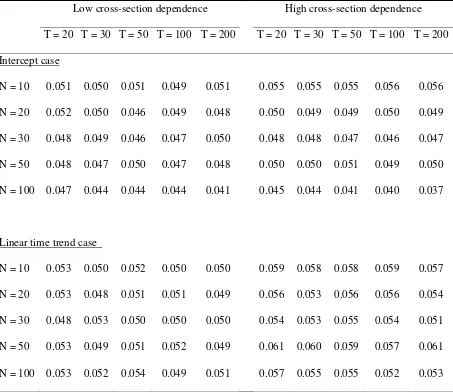
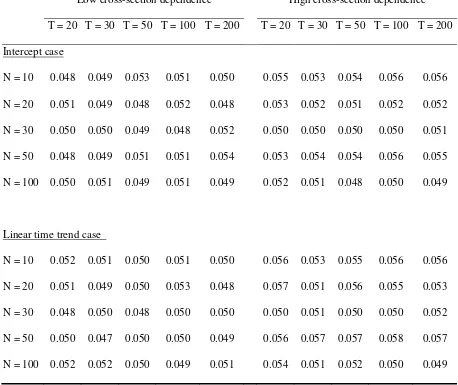
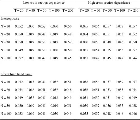
Tables II through IV present the simulation results in the case where ft has
heteroskedasticity. Table II shows the case of the unconditional heteroskedasticity, and
Tables III and IV indicate the case of ARCH(1) with low and high volatility persistence,
respectively. As these tables suggest, irrespective of the difference in type of
heteroskedasticity and in the parameter settings, the computed values of the empirical
size are almost the same as the 5% nominal size. This finding implies that Pesaran’s
(2007) CIPS test is substantially robust for the presence of conditional and
unconditional heteroskedasticity in ft.
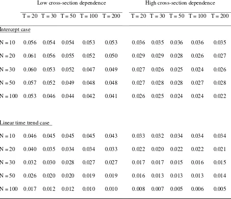
Tables V through VII report the results in the case where εithas heteroskedasticity. In
contrast to the data where ft has heteroskedasticity, size distortions are observed. As
Table V shows, CIPS test suffers from the problem of under-size distortions when the
unconditional heteroskedasticity exists in εit. The degree of the distortion tends to be
large in the case of the linear time trend model and the high cross-section dependence,
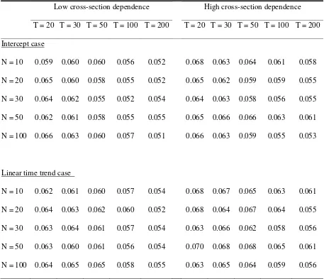
and it has a tendency to increase as N enlarges. According to Tables VI and VII, the
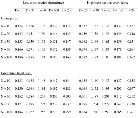
presence of ARCH(1) in εit leads to the problem of over-size distortions. Interestingly,
heteroskedasticity. Since the values of the empirical size in the low persistence case
(Table VI) are around 0.06, the degree of the distortions is not too large. However, in the
high persistence case (Table VII), the minimum value of the empirical size is 0.114, and
the maximum value is 0.273. Hence, it is clear that, in finite samples, the size
distortions of CIPS test due to the presence of ARCH(1) in εit are more serious in the
high persistence case than in the low persistence case. This property of CIPS test is
similar to that observed with the Dickey-Fuller test (Kim and Schmidt, 1993; Sjölander,
2008). Table VII indicates that, as N enlarges, the degree of the distortion increases in
the range of T =20 to T =50 or 100, and that its degree slightly decreases in more than
50 or 100
T = at arbitrary sample size N.
4. CONCLUSION
This paper used Monte Carlo simulations to analyze the small sample properties of the
panel unit root test (CIPS test) proposed by Pesaran (2007). While there are several
previous examples of work examining the small sample properties of the CIPS test, this
paper is unique for its analysis of the impacts of time-series heteroskedasticity on CIPS
test size. Numerous papers have analyzed the impacts of heteroskedasticity on the
Dickey-Fuller test and other tests for a unit root in a univariate series, but there has been
very little, if any, work done to perform the same analysis on panel unit root tests,
including the CIPS test. Analyzing the impact of heteroskedasticity on panel unit root
tests is extremely important, given the large number of economic variables with
For this paper, we considered two types of heteroskedasticity, unconditional
heteroskedasticity and ARCH, as characteristics of the unobserved common factor ft
and the idiosyncratic error term εit, and we analyzed the impacts on CIPS test size. For
ARCH, we examined cases of high and low volatility persistence separately. Our results
showed that when there is heteroskedasticity only in ft, there was almost no CIPS test
size distortion, regardless of heteroskedasticity types (unconditional or conditional) and
degree of volatility persistence. The CIPS test, therefore, could be extremely robust
versus heteroskedasticity in the unobserved common factor.
In contrast, when there is heteroskedasticity only in εit, our analysis found distortion
in the CIPS test size. Importantly, we found under-size distortion in the case of
unconditional heteroskedasticity and, conversely, over-size distortion in the case of
ARCH. Furthermore, we observed a tendency for over-size distortion to moderate with
low volatility persistence in the ARCH process and exaggerate with high volatility
persistence. It follows, then, that the problem of under-rejection of the null hypothesis
emerges when there is unconditional heteroskedasticity in εit—for example, in the
form of a distribution shift due to a structural change—and serious over-rejection
emerges when εit is characterized by an ARCH process with high volatility
persistence.
REFERENCES
Breitung J, Pesaran MH. 2008. Unit roots and cointegration in panels. In The econometrics of panel
data: fundamentals and recent developments in theory and practice, Matyas L, Sevestre P (eds).
Springer: Heidelberg.
Cerasa A. 2008. CIPS test for unit root in panel data: further Monte Carlo results. Economics
Bulletin3: 1-13.
Choi I. 2006. Nonstationary panels. In Palgrave Handbooks of Econometrics, vol. 1, Mills TC,
Patterson K (eds). Palgrave Macmillan: Basingstoke.
De Silva S, Hadri K, Tremayne AR. 2009. Panel unit root tests in the presence of cross-sectional
dependence: finite sample performance and an application. Econometrics Journal12: 340-366.
Doornik JA. 2006. Ox: An Object-Oriented Matrix Programming Language. Timberlake
Consultants: London.
Hamori S, Tokihisa A. 1997. Testing for a unit root in the presence of a variance shift. Economics
Letters57: 245-253.
Im KS, Pesaran MH, Shin Y. 2003. Testing for unit roots in heterogeneous panels. Journal of
Econometrics115: 53-74.
Kim K, Schmidt P. 1993. Unit root tests with conditional heteroskedasticity. Journal of
Econometrics59: 287-300.
Levin A, Lin F, Chu C. 2002. Unit root tests in panel data: asymptotic and finite-sample properties.
Maddala GS, Wu S. 1999. A comparative study of unit root tests with panel data and a new simple
test. Oxford Bulletin of Economics and Statistics61: 631-652.
Moon HR, Perron B. 2004. Testing for a unit root in panels with dynamic factors. Journal of
Econometrics122: 81-126.
O’Connel PGJ. 1998. The overvaluation of purchasing power parity. Journal of International
Economics44: 1-19.
Pesaran MH. 2006. Estimation and inference in large heterogeneous panels with a multifactor error
structure. Econometrica74: 967-1012.
Pesaran MH. 2007. A simple panel unit root test in the presence of cross-section dependence.
Journal of Applied Econometrics22: 265-312.
Phillips PCB, Sul D. 2003. Dynamic panel estimation and homogeneity testing under cross section
dependence. Econometric Journal6: 217-259.
Sjölander P. 2008. A new test for simultaneous estimation of unit roots and GARCH risk
in the presence of stationary conditional heteroscedasticity disturbances. Applied
Financial Economics18: 527-558.
Strauss J, Yigit T. 2003. Shortfalls of panel unit root testing. Economics Letters 81:
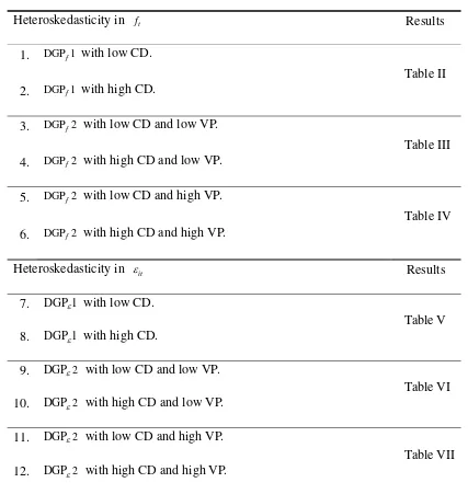
Table I. Data generating process
Heteroskedasticity in ft Results
[image:17.595.84.511.167.618.2]1. DGP 1f with low CD.
Table II 2. DGP 1f with high CD.
3. DGP 2f with low CD and low VP.
Table III 4. DGP 2f with high CD and low VP.
5. DGP 2f with low CD and high VP.
Table IV 6. DGP 2f with high CD and high VP.
Heteroskedasticity in εit Results
7. DGP 1ε with low CD.
Table V 8. DGP 1ε with high CD.
9. DGPε2 with low CD and low VP.
Table VI
10. DGPε2 with high CD and low VP.
11. DGPε2 with low CD and high VP.
Table VII
12. DGPε2 with high CD and high VP.
Note: The DGP 1f , DGP 2f , DGP 1ε , and DGPε2 are defined in Equations (12) through
(15). CD and VP designate the cross-section dependence (CD) and the volatility persistence
Table II. Empirical size of CIPS tests with unconditional heteroskedasticity in ft
Low cross-section dependence High cross-section dependence
T = 20 T = 30 T = 50 T = 100 T = 200 T = 20 T = 30 T = 50 T = 100 T = 200
Intercept case
N = 10 0.051 0.050 0.051 0.049 0.051 0.055 0.055 0.055 0.056 0.056
N = 20 0.052 0.050 0.046 0.049 0.048 0.050 0.049 0.049 0.050 0.049
N = 30 0.048 0.049 0.046 0.047 0.050 0.048 0.048 0.047 0.046 0.047
N = 50 0.048 0.047 0.050 0.047 0.048 0.050 0.050 0.051 0.049 0.050
N = 100 0.047 0.044 0.044 0.044 0.041 0.045 0.044 0.041 0.040 0.037
Linear time trend case
N = 10 0.053 0.050 0.052 0.050 0.050 0.059 0.058 0.058 0.059 0.057
N = 20 0.053 0.048 0.051 0.051 0.049 0.056 0.053 0.056 0.056 0.054
N = 30 0.048 0.053 0.050 0.050 0.050 0.054 0.053 0.055 0.054 0.051
N = 50 0.053 0.049 0.051 0.052 0.049 0.061 0.060 0.059 0.057 0.061
N = 100 0.053 0.052 0.054 0.049 0.051 0.057 0.055 0.055 0.052 0.053
Note: The empirical size (one-sided lower probability) of CIPS test is computed at the critical
Table III. Empirical size of CIPS tests with ARCH(1) in ft: low volatility persistence
Low cross-section dependence High cross-section dependence
T = 20 T = 30 T = 50 T = 100 T = 200 T = 20 T = 30 T = 50 T = 100 T = 200
Intercept case
N = 10 0.048 0.049 0.053 0.051 0.050 0.055 0.053 0.054 0.056 0.056
N = 20 0.051 0.049 0.048 0.052 0.048 0.053 0.052 0.051 0.052 0.052
N = 30 0.050 0.050 0.049 0.048 0.052 0.050 0.050 0.050 0.050 0.051
N = 50 0.048 0.049 0.051 0.051 0.054 0.053 0.054 0.054 0.056 0.055
N = 100 0.050 0.051 0.049 0.051 0.049 0.052 0.051 0.048 0.050 0.049
Linear time trend case
N = 10 0.052 0.051 0.050 0.051 0.050 0.056 0.053 0.055 0.056 0.056
N = 20 0.051 0.049 0.050 0.053 0.048 0.057 0.051 0.056 0.055 0.053
N = 30 0.048 0.050 0.048 0.050 0.050 0.050 0.051 0.050 0.050 0.052
N = 50 0.050 0.047 0.050 0.050 0.049 0.056 0.057 0.057 0.058 0.057
N = 100 0.052 0.052 0.050 0.049 0.051 0.054 0.051 0.052 0.050 0.049
Note: The empirical size (one-sided lower probability) of CIPS test is computed at the critical
Table IV. Empirical size of CIPS tests with ARCH(1) in ft: high volatility persistence
Low cross-section dependence High cross-section dependence
T = 20 T = 30 T = 50 T = 100 T = 200 T = 20 T = 30 T = 50 T = 100 T = 200
Intercept case
N = 10 0.052 0.050 0.052 0.050 0.050 0.055 0.056 0.057 0.057 0.057
N = 20 0.050 0.049 0.048 0.049 0.048 0.054 0.053 0.051 0.053 0.052
N = 30 0.050 0.049 0.050 0.047 0.052 0.050 0.050 0.048 0.046 0.050
N = 50 0.049 0.049 0.050 0.050 0.050 0.055 0.054 0.055 0.055 0.057
N = 100 0.052 0.047 0.047 0.049 0.045 0.051 0.047 0.045 0.047 0.044
Linear time trend case
N = 10 0.052 0.047 0.049 0.052 0.051 0.058 0.056 0.057 0.059 0.057
N = 20 0.054 0.048 0.051 0.052 0.048 0.056 0.051 0.053 0.055 0.054
N = 30 0.049 0.052 0.049 0.048 0.049 0.051 0.052 0.051 0.049 0.049
N = 50 0.050 0.049 0.049 0.049 0.051 0.059 0.057 0.056 0.055 0.058
N = 100 0.053 0.049 0.049 0.050 0.049 0.055 0.052 0.048 0.046 0.046
Note: The empirical size (one-sided lower probability) of CIPS test is computed at the critical
Table V. Empirical size of CIPS tests with unconditional heteroskedasticity in εit
Low cross-section dependence High cross-section dependence
T = 20 T = 30 T = 50 T = 100 T = 200 T = 20 T = 30 T = 50 T = 100 T = 200
Intercept case
N = 10 0.056 0.054 0.054 0.053 0.053 0.036 0.035 0.036 0.036 0.035
N = 20 0.061 0.056 0.055 0.052 0.050 0.029 0.029 0.028 0.026 0.027
N = 30 0.060 0.053 0.052 0.047 0.049 0.027 0.026 0.025 0.024 0.026
N = 50 0.057 0.052 0.049 0.048 0.048 0.027 0.028 0.028 0.027 0.028
N = 100 0.053 0.046 0.044 0.042 0.041 0.026 0.025 0.024 0.024 0.022
Linear time trend case
N = 10 0.046 0.045 0.045 0.045 0.043 0.033 0.032 0.034 0.034 0.034
N = 20 0.040 0.035 0.034 0.034 0.033 0.022 0.020 0.022 0.022 0.021
N = 30 0.032 0.030 0.028 0.027 0.027 0.017 0.017 0.015 0.016 0.015
N = 50 0.026 0.020 0.020 0.019 0.019 0.016 0.013 0.013 0.013 0.014
N = 100 0.017 0.012 0.012 0.010 0.010 0.008 0.007 0.005 0.006 0.005
Note: The empirical size (one-sided lower probability) of CIPS test is computed at the critical
Table VI. Empirical size of CIPS tests with ARCH(1) in εit: low volatility persistence
Low cross-section dependence High cross-section dependence
T = 20 T = 30 T = 50 T = 100 T = 200 T = 20 T = 30 T = 50 T = 100 T = 200
Intercept case
N = 10 0.059 0.060 0.060 0.056 0.052 0.068 0.063 0.064 0.061 0.058
N = 20 0.065 0.060 0.058 0.055 0.052 0.065 0.062 0.059 0.059 0.055
N = 30 0.064 0.062 0.055 0.052 0.054 0.064 0.063 0.058 0.056 0.055
N = 50 0.062 0.061 0.058 0.055 0.055 0.065 0.066 0.066 0.063 0.061
N = 100 0.066 0.063 0.060 0.057 0.051 0.066 0.063 0.059 0.055 0.053
Linear time trend case
N = 10 0.062 0.061 0.060 0.057 0.054 0.068 0.067 0.065 0.063 0.061
N = 20 0.064 0.063 0.062 0.060 0.052 0.068 0.064 0.067 0.064 0.055
N = 30 0.063 0.064 0.061 0.057 0.054 0.063 0.066 0.062 0.058 0.056
N = 50 0.063 0.060 0.061 0.056 0.054 0.070 0.068 0.068 0.065 0.061
N = 100 0.064 0.065 0.065 0.058 0.055 0.063 0.065 0.064 0.059 0.056
Note: The empirical size (one-sided lower probability) of CIPS test is computed at the critical
Table VII. Empirical size of CIPS tests with ARCH(1) in εit: high volatility persistence
Low cross-section dependence High cross-section dependence
T = 20 T = 30 T = 50 T = 100 T = 200 T = 20 T = 30 T = 50 T = 100 T = 200
Intercept case
N = 10 0.124 0.126 0.132 0.122 0.114 0.132 0.132 0.138 0.132 0.127
N = 20 0.145 0.151 0.150 0.146 0.135 0.159 0.159 0.158 0.159 0.148
N = 30 0.153 0.159 0.158 0.151 0.147 0.162 0.166 0.162 0.159 0.151
N = 50 0.166 0.171 0.175 0.172 0.158 0.174 0.177 0.183 0.178 0.164
N = 100 0.186 0.185 0.183 0.180 0.163 0.182 0.183 0.185 0.181 0.162
Linear time trend case
N = 10 0.123 0.135 0.143 0.147 0.141 0.135 0.140 0.152 0.157 0.155
N = 20 0.150 0.164 0.184 0.192 0.183 0.164 0.172 0.193 0.203 0.197
N = 30 0.152 0.184 0.201 0.207 0.203 0.161 0.189 0.203 0.212 0.212
N = 50 0.171 0.195 0.222 0.238 0.232 0.185 0.204 0.228 0.242 0.238
N = 100 0.184 0.222 0.252 0.273 0.259 0.184 0.220 0.250 0.265 0.261
Note: The empirical size (one-sided lower probability) of CIPS test is computed at the critical