Septic B Spline Solution of Fifth Order Boundary Value Problems

http://dx.doi.org/10.4236/jamp.2016.48149

Septic B-Spline Solution of Fifth-Order

Boundary Value Problems

Bin Lin

School of Mathematics and Computation Science, Lingnan Normal University, Zhanjiang, China

Received 8 July 2016; accepted 6 August 2016; published 9 August 2016 Copyright © 2016 by author and Scientific Research Publishing Inc.

This work is licensed under the Creative Commons Attribution International License (CC BY). http://creativecommons.org/licenses/by/4.0/

Abstract

A numerical method based on septic B-spline function is presented for the solution of linear and nonlinear fifth-order boundary value problems. The method is fourth order convergent. We use the quesilinearization technique to reduce the nonlinear problems to linear problems and use B-spline collocation method, which leads to a seven nonzero bands linear system. Illustrative ex-ample is included to demonstrate the validity and applicability of the proposed techniques.

Keywords

Septic B-Spline Function, Fifth-Order Boundary Value Problems, B-Spline Collocation Method, Nonlinear Problems

1. Introduction

Consider the following fifth-order boundary value problem.

( )

( )5

_{( ) ( ) ( )}

_{( )}

,

Ly x = y x +p x y x = f x c< <x d (1) With boundary conditions

( )

( )

_{( )}

( )

_{( )}

( )

( )

_{( )}

( )

_{( )}

1 2

0 1 2

1 2

3 4 5

, , ,

, ,

y c y c y c

y d y d y d

α α α

α α α

= = =

= = = (2)

where αi

(

i=0,1, 2, 3, 4, 5

)

are known real constants, p x

( )

and f x

( )

are continuous on

[ ]

c d, . This

B-spline functions based on piece polynomials are useful wavelet basis functions, the resulting matrices are sparse, but always, banded. And that possess attractive properties: piecewise smooth, compact support, symme-try, rapidly decaying, differentiability, linear combination, B-splines were introduced by Schoenberg in 1946 [6]. Up to now, B-spline approximation method for numerical solutions has been researched by various researchers [7]-[14].

In this paper, the septic B-spline function is used as a basis function and the B-spline collocation method is studied to solve the linear and nonlinear fifth-order boundary value problems. The method is fourth order con-vergent. We use the quesilinearization technique to reduce the nonlinear problems to linear problems. The present method is tested for its efficiency by considering two examples.

2. Septic B-Spline Interpolation

An arbitrary Nth order spline function with compact support of N. It is a concatenation of N sections of (N-1)th order polynomials, continuous at the junctions or “knots”, and gives continuous (N-1)th derivatives at the junc-tions.

Let

{ }

xi iN=₀ be a uniform partition of

[ ]

c d, such that xi = +c ih, i=0,1, 2,,N, where h=

(

d−c

)

N. Let the septic B-spline function φi

( )

x with knots at the points xi be given by

( )

(

)

[

]

(

)

(

)

[

]

(

)

(

)

(

)

7

4 4 3

7 7

4 3 3 2

7 7

4 3 2

7

,

8 ,

8 28

1

i i i

i i i i

i i i

i

x x x x x

x x x x x x x

x x x x x x

x h φ − − − − − − − − − − − ∈ − − − ∈ − − − + − =

[

]

(

)

(

)

(

)

(

)

[

]

(

)

(

)

(

)

(

)

[

]

(

)

(

)

(

)

7 2 1

7 7 7 7

4 3 2 1 1

7 7 7 7

4 3 2 1 1

7 7 7

4 3 2 1

,

8 28 56 ,

8 28 56 ,

8 28 ,

i i

i i i i i i

i i i i i i

i i i i i

x x x

x x x x x x x x x x x

x x x x x x x x x x x

x x x x x x x x x

− − − − − − − + + + + + + + + + ∈ − − − + − − − ∈ − − − + − − − ∈ − − − + − ∈

[

]

(

)

(

)

[

]

(

)

[

]

2 7 7

4 3 2 3

7

4 3 4

8 ,

,

0

i i i i

i i i

x x x x x x x

x x x x x

+ + + + + + + + − − − ∈ − ∈ otherwise                   (3)

The set of splines

{

φ φ φ φ φ₋₃, ₋₂, ₋₁, ₀, ₁,⋅⋅⋅,φ φ_N, _N+1,φ_N+2,φ_N+3

}

forms a basis for the functions defined over

[

c d,

]

. The values of φ_i

( )

x and its derivatives are as shown inTable 1.

We seek the approximation S x

( )

to the exact solution y x

( )

, which uses these septic B-splines:

( )

3

( )

3 N

i i i

S x aφ x

+

=−

=

∑

(4)

which satisfies the following interpolation conditions:

( )

( )

(

)

( )

_{( )}

( )

_{( )}

( )

_{( )}

( )

_{( )}

( )

_{( )}

( )

_{( )}

( )

_{( )}

( )

_{( )}

1 1 2 2

1 1 2 2

, 0,1, 2, ,

, ,

, ,

i i

s x y x i n

s c y c s c y c

s d y d s d y d

 = =  _{= =}   = =   (5)

where ai are unknown real coefficients.

Using the septic B-spline function Equation (3) and the approximate solution Equation (4), the nodal values

( )

j

S x and S( )5

( )

xj at the node xj are given in terms of element parameters by

( )

j j3 120 j2 1191 j1 2416 j 1191 j1 120 j 2 j3

S x =a− + a− + a− + a + a+ + a+ +a+ (6)

( )5

( )

(

)

3 2 1 1 2 3

5 2520

4 5 5 4

j j j j j j j

S x a a a a a a

h − − − + + +

[image:3.595.86.541.96.255.2]

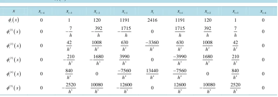
Table 1. The values of φ_i

( )

x and its derivatives with knots.

x xi−4 xi−3 xi−2 xi−1 xi xi+1 xi+2 xi+3 xi+4

( )

i x

φ 0 1 120 1191 2416 1191 120 1 0

( )1_{( )}

i x

φ 0 7

h

− 392

h

− 1715

h

− 0 1715

h

392

h

7

h 0

( )2_{( )}

i x

φ 0 2

42 h 2 1008 h 2 630 h 2 3360 h − 2 630 h 2 1008 h 2 42 h 0

( )3_{( )}

i x

φ 0 3

210 h − 3 1680 h − 3 3990

h 0 3

3990 h − 3 1680 h 3 210 h 0

( )4_{( )}

i x

φ 0 4

840

h 0 4

7560 h − 4 13440 h 4 7560 h −

0 4 840

h 0

( )5_{( )}

x

φ 0 5

2520 h − 5 10080 h 5 12600 h

− 0 5

12600 h 5 10080 h − 5 2520 h 0

From Equations (4)-(7), we have

( )

( )

( )

( )

( )

( )

( )

( )

( )

( )

( )

( )

( )

( )

(

)

5 5 5 5 5 5 5

3 2 1 1 2 3

3 2 1 1 2 3

5

120 1191 2416 1191 120

2520

4 5 5 4 ,

j j j j j j j

j j j j j j

s x s x s x s x s x s x s x

y y y y y y

h

− − − + + +

− − − + − + +

+ + + + + +

= − + − + + (8)

Using operator notations Ey x

( )

= y x

(

+h Dy x

)

,

( )

=y x Iy x′

( ) ( )

, = y x E

( )

, =ehD, we obtain

( )5

( )

3 2 1 1 2 3

5 3 2 1 1 2 3

2520 4 5 5 4

120 1191 2416 1191 120

j j

E E E E E E

s x y

h E E E I E E E

− − − + + +

− − − + + +

 − + − + − + 

= _{ }

+ + + + + +

  (9)

Expanding them in powers of hD, we obtain

( )5

( )

( )5

( )

4 ( )9

( )

59 6 ( )11

( )

259 8 ( )13

( )

( )

10

240 15120 226800

j j j j j

h h h

s x =y x − y x − y x + y x +O h (10)

Hence we get

( )

j j3 120 j2 1191 j1 2416 j 1191 j1 120 j2 j3

y x =a− + a− + a− + a + a+ + a+ +a+ (11)

( )5

( )

(

)

( )

4

3 2 1 1 2 3

5 2520

4 5 5 4

j j j j j j j

y x a a a a a a O h

h − − − + − + +

= − + − + + + (12)

3. Spline Collocation Method

3.1. Linear Problems

From Equation (1) and Equation (12), we can get

(

)

( )

(

)

4

3 2 1 1 2 3

5

3 2 1 1 2 3

2520

4 5 5 4

120 1191 2416 1191 120

j j j j j j

j j j j j j j j j

a a a a a a O h

h

p a a a a a a a f

− − − + + +

− − − + + +

− + − + − + +

+ + + + + + + =

(13)

Using the boundary conditions and by neglecting the error of Equation (13), we can obtain following linear equations

3 2 1

5 5 5

1 2 3

5 5 5

2520 10080 12600

120 1191

12600 10080 2520

2416 1191 120

j j j j j j

j j j j j j j j j

p a p a p a

h h h

p a p a p a p a f

h h h

Or

Ba=r (15) where

2 2 2 2 2 2 2

4,1 4,2 4,3 4,4 4,5 4,6 4,7

5,2 5,3 5,4 5,5 5,6 5,7 5,8

4 ,1 4 ,2

1 120 1191 2416 1191 120 1 0 0

7 392 1715 1715 392 7

0 0 0

42 1008 630 3360 630 1008 42

0 0

0 0

0 0

0 0 _{N N N}

h h h h h h

h h h h h h h

LB LB LB LB LB LB LB

LB LB LB LB LB LB LB

B

LB_{+ +} LB_{+ +}

− − −

−

=





  

         

 4 ,3 4 ,4 4 ,5 4 ,6 4 ,7

2 2 2 2 2 2 2

0 0 1 120 1191 2416 1191 120 1

7 392 1715 1715 392 7

0 0 0

42 1008 630 3360 630 1008 42

0 0

N LB N N LB N N LB N N LB N N LB N N

h h h h h h

h h h h h h h

+ + + + + + + + + +

 

 

 

 

 

 

 

 

 

 

 

 

 

 

 

 _{− − −} 

 

 

 ₋ 

 

 

 



(

)

T

3, 2, 1, , 0 1, , N, N1, N 2, N 3

a= a₋ a₋ a₋ a a ⋅⋅⋅a a ₊ a ₊ a ₊

( )

( )

_{( )}

( )

_{( ) ( ) ( )}

_{( ) ( )}

( )

_{( )}

( )

_{( )}

(

)

T

1 2 1 2

0 1

, , , , , , ,N , ,

r= y c y c y c f x f x ⋅⋅⋅ f x y d y d y d

where

(

)

( )

4 ,1 5 4 ,2 5 4 ,3 5

4 ,4 4 ,5 5 4 ,6 5

4 ,7 5

2520 10080 12600

, 120 , 1191

12600 10080

2416 , 1191 , 120

2520

, , , 0,1, 2, ,

k k k k k k k k k

k k k k k k k k k

k k k k k k

LB p LB p LB p

h h h

LB p LB p LB p

h h

LB p p p a kh f f x k N

h

+ + + + + +

+ + + + + +

+ +

= − + = + = − +

= = + = − +

= + = + = = _

T denoting transpose.

In which B is a square matrix of order N + 7 with seven nonzero bands. Since B is nonsingular, after solving the linear system Equation (15) for a−3,a−2,⋅⋅⋅,aN+2,aN+3, we can obtain the septic spline approximate

solution

( )

( )

3 3 N

i i i

S x aφ x

+

=−

=

∑

with the accuracy being O h

( )

4 .

3.2. Nonlinear Problems

Consider the nonlinear fifth order boundary value problem

( )5

_{( )}

₍

₎

, ,

y x =F x y y′ (16) with boundary conditions

( )

( )

_{( )}

( )

_{( )}

( )

( )

_{( )}

( )

_{( )}

1 2

0 1 2

1 2

3 4 5

, , ,

, ,

y c y c y c

y d y d y d

α α α

α α α

= = =

= = = (17)

( )

( )

(

)

(

( )

)

( )

(

)

( )

( )

( )

(

)

5 1 1 1 , , , , , k k

k k k k k k

k

x y x y

F F

y F x y y F y y y y y y

y + y +

+ ∂  ∂  ′ ′ ′ ′ = ≈ +_{ } − +_{ } − ′ ∂ ∂

    (18)

Equation (18) can be rewritten as

( )5

_{( )}

( )1

_{( )}

_{( )}

1 1 1 ,

k k k k k k

y+ +q x y+ +p x y+ = f x c< <x d (19) where

( )

( )

( )

( )

( )

(

( )

)

( ) ( )

( )

, , , , , , , k k k k k k

x y x y

k k k k k

x y x y

F F

q x p x

y y

F F

f x F y y y y

y y ∂  ∂  = −_{ } = −_{ } ′ ∂ ∂     ∂  ∂  ′ ′ = −_{ } −_{ } ′ ∂ ∂    

Equation (19) once the initial values (k = 0, q_k

( )

x , p_k

( )

x , f_k

( )

x ) has been computed from the initial conditions, Equation (19) becomes into a linear equations with constant coefficients. Equation (19) can be solved by using iterative method.

Subject to the boundary conditions

( )

( )

_{( )}

( )

_{( )}

( )

( )

_{( )}

( )

_{( )}

1 2

1 0 1 1 1 2

1 2

1 3 1 4 1 5

, , ,

, ,

k k k

k k k

y c y c y c

y d y d y d

α α α

α α α

+ + +

+ + +

= = =

= = = (20)

Instead of solving nonlinear problem (16) with boundary conditions (17), we solve a sequence of linear prob-lems (19) with boundary conditions (20), we consider yk+1

( )

x as the numerical solution to nonlinear problem

(16) with boundary conditions (17).

4. Computation of Error

The relative error of numerical solution is given by

( )

( )

(

)

( )

(

)

2 1 2 1 N i i i r N i i

S x y x

E y x = = − =

∑

∑

(21)

The pointwise errors are given by

( )

i

( ) ( )

i i

E x = S x −y x (22) The maximum pointwise errors are given by

( )

( )

0 max N i i i N

E y x S x

≤ ≤

= − (23)

5. Numerical Tests

In the section, we illustrate the numerical techniques discussed in the previous section by the following prob-lems.

Example 1. Consider the following equation [15]-[17]:

( )

_{( ) ( )}

_{( )}

( )

(

)

5

, 0 1 15 10 e ,x

y x y x f x x

f x x

− = ≤ ≤

= − +

With boundary conditions

( )

( )

_{( )}

( )

_{( )}

( )

( )

_{( )}

( )

_{( )}

1 2

1 2

0 0, 0 1, 0 0,

1 0, 1 e, 1 4e

y y y

y y y

= = =

The exact solution is given by

( ) (

1

)

ex

y x =x −x

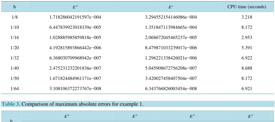
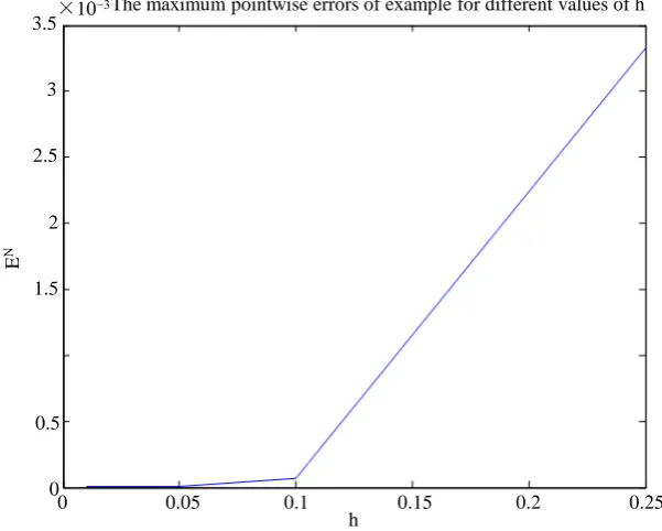
The numerical results are shown inTable 2, the comparison of maximum absolute errors are given byTable 3. The relative errors for different values of h are seen inFigure 1. The pointwise errors of example are given in

Figure 2. The maximum pointwise errors for different values of h are given inFigure 3.

[image:6.595.84.541.200.403.2]

Example 2. Consider the following nonlinear equation [15] [18] [19]. Table 2. Maximum absolute errors, relative error for example 1.

h _EN _Er _{CPU time (seconds)}

1/8 1.718286042191597e−004 3.294552154146086e−004 3.218 1/10 6.447839923018339e−005 1.351847113984665e−004 8.172 1/16 1.028885985859818e−005 2.068672045465237e−005 2.953 1/20 4.192815893866442e−006 8.479871033239017e−006 5.391 1/32 6.368030709968942e−007 1.296221338426021e−006 6.922 1/40 2.475231232201836e−007 5.045908672756208e−007 8.688 1/50 1.671824484961171e−007 3.420027458407504e−007 8.172 1/64 3.108106372273767e−008 6.343766826003454e−008 6.921 Table 3. Comparison of maximum absolute errors for example 1.

h

N

E _EN _EN _EN

Our method Caglar et al. [15] Shahid.et al. [16] Khan et al. [17]

[image:6.595.86.520.210.706.2]

1/10 6.447839923018339E−5 0.1570 2.259E−4 4.025E−3 1/20 4.192815893866442E−6 0.0747 1.33E−5 3.911E−3 1/40 2.475231232201836E−7 0.0208 5.2812E−7 1.145E−2

Figure 1. The relative errors of example 1 for different values of h. h

0 0.05 0.1 0.15 0.2 0.25

E

r

×10−3 The relative errors of example for different values of h

[image:6.595.176.458.458.707.2]

[image:7.595.186.462.83.308.2]

Figure 2. The pointwise errors of example 1.

Figure 3. The maximum pointwise errors of example 1 for different values of h.

( )5

_{( )}

2

_{( )}

e x , 0 1

y x = − y x ≤ ≤x

With boundary conditions

( )

( )

_{( )}

( )

_{( )}

( )

( )

_{( )}

( )

_{( )}

1 2

1 2

0 0 0 1

1 1 1 e

y y y

y y y

= = =

= = =

The exact solution is given by y x

( )

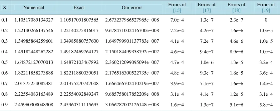
=ex.

Comparison of numerical results and pointwise errors are given inTable 4. The numerical result is found in good agreement with exact solution.

The pointwise errors of example

exact approximation

0 0.1 0.2 0.3 0.4 0.5 0.6 0.7 0.8 0.9 1 0.45

0.4

0.35

0.3

0.25

0.2

0.15

0.1

0.05

0

−0.05

The maximum pointwise errors of example for different values of h ×10−3

3.5

3

2.5

2

1.5

0.5

0

h

0 0.05 0.1 0.15 0.2 0.25

E

[image:7.595.162.463.326.567.2]

[image:8.595.89.538.101.279.2]

Table 4. Example 2. Comparison of results and pointwise errors.

X Numerical Exact Our errors Errors of

[15]

Errors of

[17]

Errors of

[18]

Errors of

[19]

0.1 1.10517089134327 1.10517091807565 2.673237986527965e−008 7.0e−4 1.3e−7 2.3e−7 0 0.2 1.22140266137546 1.22140275816017 9.678471002416700e−008 7.2e−4 4.2e−7 1.6e−6 1.0e−5 0.3 1.34985864259601 1.34985880757600 1.649799901137783e−007 4.1e−4 7.2e−7 4.6e−6 1.0e−5 0.4 1.49182448262282 1.49182469764127 2.150184499338792e−007 4.6e−4 9.4e−7 8.9e−6 1.0e−4 0.5 1.64872127070013 1.64872103467892 2.360212099095094e−007 4.7e−4 1.0e−6 1.3e−5 3.2e−4 0.6 1.82211858273888 1.82211880039051 2.176516300522735e−007 4.8e−4 9.3e−7 1.6e−5 3.6e−4 0.7 2.01375254082381 2.01375270747048 1.666466702410219e−007 3.9e−4 7.1e−7 1.6e−6 1.4e−4 0.8 2.22554083163489 2.22554092849247 9.685758017852209e−008 3.1e−4 4.1e−7 1.2e−5 3.1e−4 0.9 2.45960308048908 2.45960311115695 3.066787002126148e−008 1.6e−4 1.3e−7 5.1e−6 5.8e−4

6. Conclusion

In the paper, the fifth-order boundary value problems are solved by means of septic B-splines collocation me-thod. We use the quesilinearization technique to reduce the nonlinear problems to linear problems and reduce a boundary value problem to the solution of algebraic equations with seven nonzero bands. The numerical results show that the present method is relatively simple to collocate the solution at the mesh points and easily carried out by a computer and approximates the exact solution very well.

Acknowledgements

The authors would like to thank the editor and the reviewers for their valuable comments and suggestions to im-prove the results of this paper. This work was supported by the Natural Science Foundation of Guangdong (2015A030313827).

References

[1] Karageorghis, A., Phillips, T.N. and Davies, A.R. (1988) Spectral Collocation Methods for the Primary Two-Point Boundary Value Problem in Modeling Viscoelastic Flows. International Journal for Numerical Methods in Engineer-ing, 26, 805-813. http://dx.doi.org/10.1002/nme.1620260404

[2] Davies, A.R., Karageorghis, A. and Phillips, T.N. (1988) Spectral Galerkin Methods for the Primary Two-Point Boun-dary Value Problem in Modeling Viscoelastic Flows. International Journal for Numerical Methods in Engineering, 26, 647-662. http://dx.doi.org/10.1002/nme.1620260309

[3] Caglar, H.N., Caglar, S.H. and Twizell, E.H. (1999) The Numerical Solution of Fifth-Order Boundary Value Problems with Sixth-Degree B-Spline Functions. Applied Mathematics Letters, 12, 25-30.

http://dx.doi.org/10.1016/S0893-9659(99)00052-X

[4] Siddiqi, S.S. and Akram, G. (2006) Solutions of Fifth Order Boundary Value Problems Using Nonpolynomial Spline Technique. Applied Mathematics and Computation, 175, 1574-1581. http://dx.doi.org/10.1016/j.amc.2005.09.004 [5] Lamnii, A., Mraoui, H., Sbibih, D. and Tijini, A. (2008) Sextic Spline Solution of Fifth Order Boundary Value

Prob-lems. Mathematics and Computers in Simulation, 77, 237-246. http://dx.doi.org/10.1016/j.matcom.2007.09.008 [6] De Boor, C. (1978) A Practical Guide to Splines. Springer-Verlag, pp. 54, 105.

http://dx.doi.org/10.1007/978-1-4612-6333-3

[7] Saka, B. and Dağ, I. (2007) Quartic B-Spline Collocation Method to the Numerical Solutions of the Burgers’ Equation.

Chaos, Solitons & Fractals, 32, 1125-1137. http://dx.doi.org/10.1016/j.chaos.2005.11.037

[8] Ramadan, M.A., EI-Danaf, T.S. and Alaal, F. (2005) A Numerical Solution of the Burgers’ Equation Using Septic B-Splines. Chaos, Solitons & Fractals, 26, 795-804. http://dx.doi.org/10.1016/j.chaos.2005.01.054

[10] Çağlar, H.,Çağlar, N. and Özer, M. (2009) B-Spline Solution of Non-Linear Singular Boundary Value Problems Aris-ing in Physiology. Chaos, Solitons & Fractals, 39, 1232-1237. http://dx.doi.org/10.1016/j.chaos.2007.06.007 [11] Çağlar, H., Özer, M.and Çağlar, N. (2008) The Numerical Solution of the One-Dimensional Heat Equation by Using

Third Degree B-Spline Functions. Chaos, Solitons & Fractals, 38, 1197-1201. http://dx.doi.org/10.1016/j.chaos.2007.01.056

[12] Saka, B. and Dağ, İ. (2007) Quartic B-Spline Collocation Method to the Numerical Solutions of the Burgers’ Equation.

Chaos, Solitons & Fractals, 32, 1125-1137. http://dx.doi.org/10.1016/j.chaos.2005.11.037

[13] Jain, P.C., Shankar, R. and Bhardwaj, D. (1997) Numerical Solution of the Korteweg-de Vries (KdV) Equation. Chaos,

Solitons & Fractals, 8, 943-951. http://dx.doi.org/10.1016/S0960-0779(96)00135-X

[14] Lin, B., Li, K.T. and Cheng, Z.X. (2009) B-Spline Solution of a Singularly Perturbed Boundary Value Problem Arising in Biology. Chaos, Solitons & Fractals, 42, 2934-2948. http://dx.doi.org/10.1016/j.chaos.2009.04.036

[15] Caglar, H.N., Caglar, S.H. and Twizell, E.N. (1999) The Numerical Solution of Fifth-Order Boundary Value Problems with Sixth-Degree B-Spline Functions. Applied Mathematics Letters, 12, 25-30.

http://dx.doi.org/10.1016/S0893-9659(99)00052-X

[16] Siddiqi, S.S. and Akram, G. (2007) Sextic Spline Solutions of Fifth-Order Boundary Value Problems. Applied Mathe-matics Letters, 20, 591-597. http://dx.doi.org/10.1016/j.aml.2006.06.012

[17] Khan, M. (1994) Finite Difference Solutions of Fifth-Order Boundary Value Problems. Ph.D. Thesis, Brunel Universi-ty, England.

[18] Noor, M.A. and Mohyud-Din, S.T. (2009) A New Approach to Fifth-Order Boundary Value Problems. International Journal of Nonlinear Science, 7, 143-148.

[19] Zhang, J. (2009) The Numerical Solution of Fifth-Order Boundary Value Problems by the Variational Iteration Method.

Computers & Mathematics with Applications, 58, 2347-2350. http://dx.doi.org/10.1016/j.camwa.2009.03.073

Submit or recommend next manuscript to SCIRP and we will provide best service for you:

Accepting pre-submission inquiries through Email, Facebook, LinkedIn, Twitter, etc. A wide selection of journals (inclusive of 9 subjects, more than 200 journals) Providing 24-hour high-quality service

User-friendly online submission system Fair and swift peer-review system

Efficient typesetting and proofreading procedure

Display of the result of downloads and visits, as well as the number of cited articles Maximum dissemination of your research work