Munich Personal RePEc Archive
Modelling biodiversity
Halkos, George
University of Thessaly, Department of Economics
2010
Online at
https://mpra.ub.uni-muenchen.de/39075/
Modelling biodiversity
George E. Halkos
Department of Economics, University of Thessaly
Abstract
This study uses a sample of 71 countries and nonparametric quantile and partial regressions to model a number of threatened species (reptiles, mammals, fish, birds, trees, plants) in relation to various economic and environmental variables (GDPc, CO2
emissions, agricultural production, energy intensity, protected areas, population and income inequality). From the analysis and due to high asymmetric distribution of the dependent variables it seems that a linear regression is not adequate and cannot capture properly the dimension of the threatened species. We find that using OLS instead of non-parametric techniques over- or under-estimates the parameters which may have serious policy implications.
Keywords: Nonparametricquantile regression; partial regression; biodiversity.
JEL Classifications: Q57, Q20, C14, C40
Address for Correspondence Professor George Halkos
Director of Operations Research Laboratory Deputy Head
Department of Economics, University of Thessaly,
Korai 43, 38333, Volos, Greece. http://www.halkos.gr/
1. Introduction
The biological diversity (biodiversity) is a concept entailed in the modern
scientific and political terminology and in daily life with various social and economic
dimensions. After the signing of the Convention on Biological Diversity (CBD) by a
considerable number of countries (168 signatures in the 191 parties to the CBD)1 in
Rio de Janeiro in 1992, the term was recognized globally. Although there is no
common definition accepted, the term biodiversity encompasses everything from the
level of genes to species to the level of ecosystems. To be more specific, we may
distinguish four level of biodiversity in genes, species, ecosystems and functional
diversity (Turner et al. 1999).
Biodiversity and ecosystems provide us with a number of direct and indirect
social and economic benefits. The significance of biodiversity lies in its role to
preserve ecosystem resilience by guaranteeing the provision of basic ecosystem
functions under a variety of environmental situations (Perrings et al. 1995, p. 4).The
preservation of biodiversity is crucial due to the services provided by its use. These
services may be aesthetic and ecological as they are related to the normal operation
and conservation of ecosystems. They are also related to the reduction of poverty
globally as well as to medical and pharmaceutical curative methods that rely on
biological substances offered by the environment. Costanza et al. (2007) showed the
complex relationships between biodiversity and ecosystem functioning. The latter
supports ecosystem services that increase directly or indirectly human welfare.
Biodiversity is in danger due mainly to human activities. In the second half of
the 20th century, human population was doubled from 2.5 billion in 1950 to more than
6 billion in 2000. At the same time the value of economic activity increased by more
than 400% over the second half of last century (Delong, 2003). The area of natural
habitat has been reduced for a number of reasons such as conversion of lands to
agriculture, over-harvesting of fish, air and water pollution, climate change, urban
development, increasing sequence of fires in forests, etc. For these reasons the current
rates of species extinction have been dramatically increased.
Habitat loss and degradation may be considered as the main danger for
biodiversity leading to the need of finding ways of preserving natural habitats.
Governments could set biodiversity targets attempting to achieve them at minimum
cost. This would still incorporate economic realities but avoid the (controversial)
valuation of species. Alternatively governments may create protected areas like
national parks where biodiversity may be protected. Globally it is estimated that 6.4%
of the earth (with the exception of Greenland and Antarctica) is in some form of
protected area (UNDP, 2000).
Threats to the natural habitat are in general lower in the developed countries
compared to the tropical developing countries where much of the biodiversity resides.
These threats vary according to the ecosystem type. Given the threat of extinction in a
number of species and the limited capital budgets, the decision makers have to set
priorities in order to make sure that conservation of biodiversity is ensured. Thus a
complete and well-planned environmental policy requires the use of some form of
economic valuation inevitable. The economic valuation of biodiversity consists of the
effort to quantify in monetary terms the human preferences concerning the efforts to
preserve the various species.
In this study a sample of 71 countries and a number of economic and
environmental variables are used. Specifically, apart from variables like the gross
variables in other studies, a number of other variables are used for the first time like
the CO2 emissions per capita, agricultural production, energy intensity, protected
areas in every country and the GINI index of income inequality. In the same way,
variables like the number of species endangered are used for reptiles, mammals, fish,
birds, trees and plants as dependent variables.
The results are interesting as we are not relying on simple statistical and
econometric modelling methods like ordinary least squares (hereafter OLS), but we
use, for the first time to our knowledge, quantile regression with reference not to the
mean influence of the regressors on the mean of the conditional distribution of the
dependent variable but on its entire conditional distribution. Quantile regressions rely
on a number of different quantiles and estimate functional relationships between
variables for all portions of a probability distribution. It is even more useful in cases
with heterogeneous variances where OLS has serious problems (heteroskedastic error
terms). In such cases focusing only on changes in the means may underestimate or
overestimate or even fail to distinguish real nonzero changes in heterogeneous
distributions (Terrell et al. 1996; Cade et al. 1999). At the same time using quantile
regressions to model heterogeneous variances does not require any specification of
how variances changes are related to the mean. Finally, in a specific case partial
regression was used among the explanatory variables and not one but more than one
dependent variables in the same model were simultaneously considered.
The structure of this study is the following. Section 2 reviews the problem in
terms of exploring the research efforts carried out in evaluating economically
biodiversity. Section 3 presents the data used, while section 4 discusses analytically
the proposed econometric methodologies. Section 5 refers to the empirical results
2. Literature review
Biodiversity comprises the variety of types, forms, spatial arrangement,
interactions and processes from genes to species and ecosystems (Noss, 1990)
together with the evolutionary history that led to their existence (Faith, 2002).
Commonly used measures like the number of species present are fully
scale-dependent and only show a change when species have disappeared. At the same time
indices incorporating several proxy signals are quite sensitive while integrated
measures (Scholes and Biggs 2005; Hui et al. 2008) are sensitive and achievable but
they require more research in order to construct the globally robust relationships
between population data, the variation in genetics and the required ecosystem
conditions (Scholes et al. 2008). Genetically distinct populations are an important
component of biodiversity for any species (Hughes et al. 1997).
One of the main concerns of the environmental social sciences is the deep
understanding of the social and economic forces that change the environment.
Scholars have contributed to global biodiversity loss research by paying attention to
the relevance and context of species in threat to the interdisciplinary community
(Hoffman, 2004; Naidoo and Adamowicz, 2001). Due to data limitations and
reliability cross national comparisons have tackled basically the loss of land-based
species like birds and mammals. The studies mentioned only partially capture the
cumulative effects of human activity on global diversity. The proximate causes of
losses in biodiversity are probably well understood in cases of habitat destruction,
resource extraction, climate change and pollution.
But socioeconomic forces have poorly explored in biophysical phenomena.
Mikkelson et al. (2007) using OLS tested how strongly economic inequality is related
threatened species increases significantly with the GINI ratio of inequalities in
income. O’Connor et al. (2003) using a combination of biological and sociological
variables (among others GDP/c, population density, percentage of unprotected land
area and governance) in the context of a return on investment framework try to
explore the establishment of conservation priorities. They find that only a few
countries emerged as high priorities regardless of which factors were examined. On
the other hand, some countries ranked highly as priorities for conservation when
focusing solely on biological metrics, did not reach a high rank when governance,
population pressure, economic costs and conservation needs were considered.
Nunes and van den Bergh (2001) present a literature review of the economic
valuation of biodiversity according to the various available methods. Most of these
studies have been carried out in the USA and show the existence of positive social
value of biodiversity but they show simultaneously that the economic literature is
incomplete and unable to cover the full range of benefits from biodiversity.
Brody (2003) using regression analysis examines how existing biodiversity
levels affect ecosystem capabilities at the local level. On the other hand, Costanza et
al. (2007) using stepwise regression (OLS) found that biodiversity and primary
productivity are positively related in certain temperature regimes showing that a
change in biodiversity is correlated with a change in net primary production. It is
worth mentioning that the authors find nonlinear relationships for a number of
predictors which were recalculated and transformed. Similarly, Groeneveld et al.
(2005) present a spatially explicit trade-off analysis of species preservation in
agricultural areas calculating the production possibility frontiers of net monetary
In these lines, Clausen and York (2008) employ cross sectional data for
different fish species in threat and in more than 140 countries. By using a negative
binomial regression model test the environmental Kuznets curve hypothesis regarding
both the scale of economic production and urbanization. Dietz and Adger (2003), with
the use of panel and cross-sectional data, examined economic growth and biodiversity
in the EKC framework. Specifically they investigate the relationship between
economic growth, loss of biodiversity and policies to conserve biodiversity. The
authors base their effort on the idea that if economic growth causes biodiversity loss
by transforming habitat and other means, then an inverse relationship should be
expected.
3. Data used
One of the most commonly used methods of describing biodiversity of an area
is the count of species that reside in this area. Obviously a complete enumeration of
all species even in a simple square metre is impossible, as the vast majority of species
remains unknown. At the same time there are cases of existence of different
definitions for species creating different estimates of their richness. Additional
problems arise in the analysis of the geographical distribution of the various species,
the change of these distributions in time etc. The huge variety of living creatures is
ranked in multiple levels (from genes to ecosystems) making their complete
enumeration extremely difficult and in many cases infeasible.
As mentioned in this study we use economic and environmental data.
Specifically a number of variables are used as explanatory such as the Gross Domestic
Product (GDP in million $) and the per capita Gross Domestic Product (GDPc), per
(1999-2001=100), energy intensity in all economics sectors (toe per million $),
national protected areas (total number) in every country2, population (in thousands)
and the GINI index of income inequality (0= perfect equality and 100= perfect
inequality). The GINI index was calculated by the compilation of income distribution
data to extract a single number that represents the extent of income inequality within a
country.
The numbers of species endangered like reptiles, mammals, fish, birds, trees
and plants are used as dependent variables. These numbers of threatened species
include full species that are critically endangered, endangered or vulnerable but
exclude introduced species, species whose status is not sufficiently known
(characterized by IUCN as “data deficient”), those known to be extinct and those
whose status is not sufficiently known (characterized by IUCN as “not evaluated”).
The source of the data is the World Resources Database and the data refer to the year
2004 for existing species and 2006 for endangered species3. Our sample consists of 71
countries4.
2 It is worth mentioning that protected areas serve as a crucial function in protecting the earth’s
resources. However they have to cope with a number of challenges like external threats from climate change and pollution, irresponsible tourism, water resources extraction, increasing demand for land and infrastructure developments.
3 World Resources Institute (2008). EarthTrends: The Environmental Information Portal Archived
Data Tables (by Topic Area).
4 The countries used are the one with full record (no missing values). Namely, Armenia, Azerbaijan,
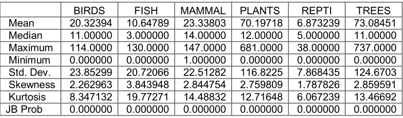
Table 1 presents the descriptive statistics of the dependent variables into
consideration. It can be seen that there are large differences between the mean and the
median (first indication of asymmetry) and differences also in standard deviations,
skewness and kurtosis. In all cases we have a positive value of skewness and the size
of kurtosis is higher than 3, which implies huge mass at high levels and short tails at
small amounts; this indicates highly asymmetric distributions. Thus the high mean
values are due to a number of observations with high percentages of species in threat
justifying the use of quantile regression. The kurtosis shows a leptokurtic type of
[image:10.595.102.494.369.484.2]distribution for the threatened species5.
Table 1: Descriptive statistics of the species in threat
Figure 1 presents the probability plots of all the species in threat assuming
normality. In all cases normality is rejected as the P-values of the Anderson-Darling
test are less than the usual statistical levels leading to the rejection of the null
hypothesis that the data follow the normal distribution.
Panama, Trinidad and Tobago, Bolivia, Brazil, Chile, Colombia, Ecuador, Paraguay, Peru, Uruguay, Venezuela, Australia.
5 According to the Box-Cox test the variables were used in levels (in most of the cases) and were not
transformed in logs.
BIRDS FISH MAMMAL PLANTS REPTI TREES
Figure 1: Probability graphical presentations of species in threat (assuming normality) 160 80 0 99.9 99 90 50 10 1 0.1 80 0 -80 99.9 99 90 50 10 1 0.1 500 0 -500 99.9 99 90 50 10 1 0.1 30 0 -30 99.9 99 90 50 10 1 0.1 80 0 -80 99.9 99 90 50 10 1 0.1 500 0 -500 99.9 99 90 50 10 1 0.1 MammalsThreat Pe rc en t 87 48 .7 BirdsThreat 87 47 .2 PlantsThreat 87 20 2 ReptiThreat 87 15 .7 4 FishThreat 87 34 .0 TreesThreat 87 21 4 Mean 23.34 StDev 22.51 N 71 AD 4.987 P-Value <0.005 MammalsThreat Mean 20.32 StDev 23.85 N 71 AD 6.381 P-Value <0.005 BirdsThreat Mean 70.20 StDev 116.8 N 71 AD 8.055 P-Value <0.005 PlantsThreat Mean 6.873 StDev 7.868 N 71 AD 5.008 P-Value <0.005 ReptiThreat Mean 10.65 StDev 20.72 N 71 AD 10.304 P-Value <0.005 FishThreat Mean 73.08 StDev 124.7 N 71 AD 8.226 P-Value <0.005 TreesThreat
Probability Plot of MammalsThrea, BirdsThreat, PlantsThreat, ...
Normal - 95% CI
4. Τhe proposed models
OLS estimates the effect of the explanatory variables on the mean of the
conditional distribution of the dependent variable. This is obviously a strong
simplification as regressors may not only determine the mean but may also influence
other parameters of the conditional distribution of the dependent variable. Quantile
regressions allow the examination of the entire conditional distribution of the
dependent variable. At the same time it is less restrictive compared to the OLS (mean)
regression as it allows the estimated parameters (slopes) to differ at different points of
[image:11.595.92.543.122.476.2]quantile regression imposes no functional form on the species endangered relationship
and it is not sensitive to the presence of extreme values (outliers), a common problem
when analysing data for developing countries. This may be justified as in quantile
regressions we minimize the residuals and not their squares as in OLS.
Quantile regressions allow the estimation of various quantile functions of a
conditional distribution where each quantile characterizes a particular (center or tail)
point of the conditional distribution. Putting together a number of different quantile
regressions gives us a more complete description of the underlying conditional
distribution.
In simple words, in the OLS application the estimated parameters represent the
change in the dependent variable caused from a unit change in the independents. The
parameters of the quantile regression estimate the change in a specific quantile of the
dependent variable due to a unitary change in the independent variable. This allows
comparisons among the quantiles in terms of how much they are influenced from
specific characteristics in relation to the other quantiles. This can be seen in the
change in the magnitude of the coefficients. Quantile regressions are extremely useful
when we face heteroskedasticity and/or no normality in the disturbance term
(Buchinsky 1998).
Let us consider the quantile regression analytically. Assume a random variable
Y with a probability distribution function given as
) Pr( )
(y Y y
F (1)
such as 0 < λ < 1 when the i quantile can be defined as the lowest y that satisfies the
condition F(y)
y F y i
Q()inf : ( ) (2)
k i
i y l Y y
F( ) ( ) (3)
Where l(z) takes the value 1 if Ζ true and 0 otherwise.
The corresponding empirical quantile is given as
} ) ( : inf{ )
( y Fn y
Qi (4)
The quantile regression extents the simple model including the explanatory variables
X assuming linear specification for the conditional quantile of the independent
variable Y given the values of the matrix P of the independent variables X.
Specifically, , ) ( )) ( |
( i j
Q (5)
where () arg (){ ( j())
j j
mm
(6)The coefficients of the quantile regression are normally distributed for large
samples (Koenker, 2005). Koenker and Bassett (1978) derive asymptotical results for
normality for the quantile regression estimates in an independently and identically
distributed (hereafter i.i.d.) formulation, showing that
(7)
where lim(i j j / ) lim(n / )
j
J
X X i X X i (8)1 1 1 ( ) ( ) ( ( )) S F f F
(9)
Where S(λ) is the quantile density function. We can calculate S
with the use of theKernel density estimator (Powell 1986, Buchinsky 1995, Jones 1992). Specifically,
1 1
1 ˆ( )
ˆ ( )
(1/ ) i j
i
i j
S
i c L c
(10) 2 1 ˆ( ( )) ( )) ~ (0, (1 ) ( ) )
where ˆjthe residuals of the quantile regression.
The kernel estimation of the density function requires the specification of the
bandwidth (Ci). If we define the coefficient vector of this procedure as
1 2
( ( ) , ( ) , , ( ) )
(11)
then i( ˆ ) ~ (0, ) (12)
where min
,
1( ) 1( )ij imum i j i jH i JH i
(13)
In the case of i.i.d. Ω becomes 0 J where 0as representative element has
)) ( ( ( )) ( ( ) , min( 1 1 j i j i j i
ij f F f F
(14)
Estimation of Ω may be done using the bootstrap method.
The test of slope equality was suggested by Koenker and Bassett (1982) and it
is a robust heteroskedasticity test
) ( ) ( ) (
:1 1 2 2
o
H
Where we have (p1)(k1) restrictions in the coefficients. The corresponding Wald
test is distributed as 2 ) 1 ( ), 1 (p k
.
Similarly, the symmetry test was proposed by Newey and Powell (1987) and
relies on the idea that if
) 2 1 ( 2 ) 1 ( ) ( (15)6
then we may estimate this restriction using the Wald test with H0 having p(k1)/2
restrictions and the Wald test is distributed as 2 2 / ) 1 (k
p
. This test compares the
estimates of the first and third quantile with the median specification.
6 As there is no clear positive relationship between the values of the quantiles and the estimated
Another suggested method in cases of highly correlated independent variables
or in the case of analysing fewer observations than variables or highly correlated
dependent variables is the partial regression (PLS). This regression estimates models
with more than one dependent variable in the same model formulation. This is
achieved by reducing the number of explanatory variables and regressing the
extracted components on the dependent variables and not on the original data. We
include more that one dependent variable when the dependent variables are correlated
between them.
5. Empirical results
Tables 2-4 present the OLS and the quantile regression estimates for the 10th,
30th, 50th, 70th, 90th quantiles. The OLS (mean) regression estimates are presented for
reasons of comparison with the quantile regression estimates. From Table 2 and
comparing the quantile (median) with the OLS (mean) estimates there are significant
differences in magnitudes. Specifically the number of endangered trees increase by
(first quantiles and then OLS estimates in parentheses) 1.72 (2.02), 2.9 (3.88), 0.03
(0.019) and 0.09 (0.007) per unit increase in agricultural production, higher income
inequality, higher level of CO2 emissions and higher population respectively.
Similarly and from table 3 it can be seen that the number of plants in threat increases
by 1.653 (2.01), 2.52 (3.92), 0.022 (0.016) and 0.0065 (0.005) per unit increase in
agricultural production, higher income inequality, higher level of CO2 emissions and
higher population.
Finally, from Table 4 we may see that the number of mammals in danger rises
by 0.09 (0.23), 0.54 (0.46), 0.025 and 0.001 (0.0009) per unit increase in agricultural
population. These comparison are more different is we compare the OLS (mean) with
the other quantilies and especially the upper ant the lower ones asa shown in Figure 3.
As a general comment we may say that the influence of the explanatory variables is
higher in the case of plants and trees endangered followed by the mammals in threat.
OLS overestimates the estimated parameters in the case of agricultural production and
income inequality and underestimates in the case of population and CO2 when we
consider trees and plants threatened with a mixture with significant differences in
magnitudes in the case of mammals endangered.
In Tables 2 and 3 the quantile regression shows that the influence of the
agricultural production on the trees and plants in threat increases as we move from the
10th to the 90th quantile with exception in the case of the 70th quantile. It is obvious
that comparing the quantile estimates with those of OLS only the 90th is comparable.
Similar conclusions can be extracted for the other variables. For the GINI index we
see an increase from the 10th till the 90th quantile. The OLS result is not comparable
with those of the quantile regression with a similarity only in the 70th quantile. In the
same table there is a negligible change in the case of the other two variables
(emissions and population) as we move across the quantiles.
In Table 4 and concerning the mammals in threat the picture is slightly
different. Income inequality is the only variable increasing as we move from the 10th
to 90th quantile. For the rest of the variables there is an unstable behaviour with
Table 2: Regression results with the trees endangered as dependent variable
Non-parametric quantile regression Explanatory
variables OLS 10
th
quantile 30
th
quantile 50
th
quantile 70
th
quantile 90
th
quantile
Constant -293.884 (-3.404) [0.0011] -54.08 (-0.76) [0.4481] -96.93 (-1.21) [0.2315] -257.54 (-3.1) [0.0029] -264.5 (-3.9) [0.0003] -259.6 (-5.3) [0.0000] Agricultural
Production/c 2.016 (2.85)
[0.0059] 0.254 (0.454) [0.6514] 0.467 (0.65) [0.5194] 1.72 (2.94) [0.0045] 1.61 (2.95) [0.0044] 2.145 (2.33) [0.0231]
GINI 3.878
(2.76) [0.0075] 0.766 (1.01) [0.3173] 1.41 (0.92) [0.1316] 2.9 (2.5) [0.0164] 3.98 (2.86) [0.0056] 5.02 (1.96) [0.0545]
CO2 0.01923
(0.999) [0.3212] 0.0007 (0.012) [0.9904] 0.024 (1.57) [0.1216] 0.03 (3.46) [0.0010] 0.023 (3.5) [0.0008] 0.004 (0.61) [0.5431]
Population 0.00684 (2.339) [0.0224] 0.00013 (0.017) [0.9868] 0.003 (0.266) [0.7912] 0.009 (7.1) [0.0000] 0.0082 (8.2) [0.0000] 0.006 (7.3) [0.0000] Quasi-LR statistic
Wald slope equality test Wald symmetric test
27.21 [0.000] 58.94 [0.002] 16 d.f. 30.17 [0.067] 10 d.f. t-statistics in parentheses; P-values in [ ]
Table 3: Regression results with the plants endangered as dependent variable
Non-parametric quantile regression Explanatory
variables OLS 10
th
quantile 30
th
quantile 50
th
quantile 70
th
quantile 90
th
Quantile
Constant -294.94 (-3.67) [0.0005] -32.96 (-0.46) [0.6453] -101.28 (-1.374) [0.1742] -234.1 (-3.009) [0.0037] -246.56 (-4.011) [0.0002] -260.78 (-4.74) [0.0000] Agricultural
Production/c 2.009 (3.044)
[0.0033] 0.154 (0.274) [0.7849] 0.536 (0.804) [0.4243] 1.653 (3.04) [0.0034] 1.485 (3.008) [0.0037] 2.131 (2.51) [0.0145]
GINI 3.92
(2.99) [0.0039] 0.504 (0.65) [0.5195] 1.4 (1.64) [0.1052] 2.521 (2.32) [0.0234] 3.872 (2.6) [0.0117] 4.824 (2.025) [0.0470]
CO2 0.016
(0.882) [0.3811] 0.0031 (0.0574) [0.9544] 0.026 (3.143) [0.0025] 0.022 (2.92) [0.0048] 0.018 (2.9) [0.0050] 0.0007 (0.11) [0.9148]
Population 0.0049 (1.81) [0.0761] -0.00008 (-0.009) [0.9925] 0.003 (0.272) [0.7866] 0.0065 (5.5) [0.0000] 0.0058 (6.3) [0.0000] 0.004 (4.51) [0.0000] Quasi-LR statistic
Wald slope equality test Wald symmetric test
[image:17.595.87.511.460.758.2]Table 4: Regression results with the mammals endangered as dependent variable
Non-parametric quantile regression Explanatory
variables OLS 10
th
quantile 30
th
quantile 50
th
quantile 70
th
quantile 90
th
quantile
Constant -43.802 (-2.742) [0.0079] -20.83 (-1.27) [0.2081] -25.22 (-1.544) [0.1274] -28.404 (-1.97) [0.0531] -48.1715 (-2.8055) [[0.0066] -45.703 (-4.391) [0.0000] Agricultural
Production/c 0.2255 (2.483)
[0.0156] 0.1146 (1.8) [0.076] 0.08123 (1.073) [0.2872] 0.0896 (1.164) [0.2488] 0.2279 (2.532) [0.0137] 0.2903 (1.7077) [0.0924]
GINI 0.4619 (1.685) [0.097] 0.1156 (0.474) [0.6374] 0.3504 (1.212) [0.2297] 0.5433 (1.919) [0.0594] 0.7351 (2.073) [0.0421] 0.848 (1.514) [0.1347]
Log CO2 5.6243
(4.0914) [0.0001] 2.6928 (1.77) [0.0821] 3.554 (2.34) [0.0224] 3.722 (2.99) [0.0040] 5.14 (2.9544) [0.0043] 5.0151 (2.894) [0.0051]
Population 0.000898 (1.6715) [0.0994] 0.00086 (2.53) [0.0139] 0.001135 (3.9953) [0.0002] 0.00099 (3.136) [0.0026] 0.000871 (2.765) [0.0074] 0.000496 (2.011) [0.0484] Quasi-LR statistic
Wald slope equality test Wald symmetric test
15.613 [0.0036]
30.153 [0.0170] 16 d.f. 16.138 [0.0950] 10 d.f. t-statistics in parentheses; P-values in [ ]
Standard errors of the quantile regressions are extracted by bootstrapping with
1000 replications. F values from Wald tests of equality of coefficients of specific
independent variables across quantiles are also presented. These Wald tests of slope
equality equal to 58.94, 38.72 and 30.153 for trees, plants and mammals in threat with
P-values equal to 0.002, 0.001 and 0.017 respectively. We may conclude that the
coefficients differ statistically across the values of the quantiles and the conditional
quantiles are not similar. At the same time, the Wald test of quantile symmetry gives
30.167, 19.88 and 16.138 with P-values equal to 0.067, 0.03 and 0.8153 respectively.
Closed related to the previous test we see that there is indication of deviation from
symmetry. As already mentioned, these results may be justified as moving from the
10th to the 90th quantile, increasing influences can be observed for the agricultural
the pollution emissions and the population. The picture is different in the case of
mammals in threat where except in the case of income inequality with an increasing
behaviour the rest of the variables present a mixture of changes.
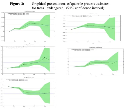
In Figure 2, the graphs of the quantile regression are done for the constant and
the explanatory variables. The OLS estimate and its 95% confidence interval are
plotted as horizontal lines. In each graph the regression coefficients show the
influence of a unit change in the independent variable (holding constant the rest of the
explanatory variables) on the specific levels of the quantiles of the dependent variable
with a 95% probability level for the confidence intervals. The constant term can be
interpreted as the estimated conditional quantile function of the endangered species
with no influence of the explanatory variables. These graphs help us to see how
changeable are those influences and show that a linear regression may be inadequate
in terms of approaching these relationships. Thus using OLS provides less
information compared to the use of quantile regressions.
Looking at figure 2 we can say that the variables agricultural production and
income inequality (with the exception of the 90th quantile) show an increasing
influence as we move from the 10th to the 90th quantile. It is interesting to mention
that in the cases of the GINI index OLS overestimates the estimated parameters till
the 70th quantile and then it underestimates the parameters. For the agricultural
production underestimation takes place till the upper quantilies (80th). In the case of
population and CO2 the picture is mixed. First OLS estimates underestimate (till the
35th) then overestimate (till the 80th) and then underestimate again. For the constant
in the case of plants and mammals endangered7. The above imply that in this kind of
environmental research we have to be careful because even if the average picture of
behaviour seems reasonable the complete separation of countries (strata) may result to
[image:20.595.93.501.191.560.2]quite different results.
Figure 2: Graphical presentations of quantile process estimates for trees endangered (95% confidence interval)
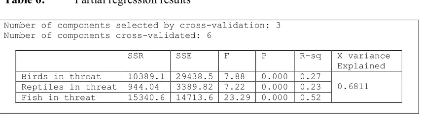
Table 5 presents the correlation coefficients among the dependent variables
(birds, fish and reptiles in danger). All the coefficients are relatively high showing
linearity among the variables. In Table 6 we may see the results of the partial
7 Due to space limitations the graphs in the cases of plants and mammals in threat are not presented but
regression among the 3 dependent variables and the 6 independent (agricultural
production, CO2 emissions, income inequality, population, GDP/c, energy intensity)8.
Table 5: Correlation coefficients of the dependent variables in the partial regression
Correlations: Birds in Threat, Reptiles in Threat, Fish in Threat Birds in Threat Fish in Threat
Fish in Threat 0.670 0.000
Reptiles in Threat 0.634 0.628 0.000 0.000 Cell Contents: Pearson correlation
P-Value
First in the results of Table 6 it can be observed that the number of
components of the optimal model (relying on the highest predicted R2) equals to three.
The table presents the analysis of variance per dependent variable and according to
the optimal model. The P-values are zero and in every case less than the usual
significance levels. In all cases there is sufficient evidence that the models are
statistically significant. The coefficient of determination is low and equals to 0.261,
0.22 and 0.51 for the birds, reptiles and fish in danger respectively.
The column X-variance shows the percentage of variance of the independent
variables which is explained by the model. In our case, the three components explain
[image:21.595.86.514.170.277.2]68.11% of the variance of the independent variables.
Table 6: Partial regression results
Number of components selected by cross-validation: 3 Number of components cross-validated: 6
SSR SSE F P R-sq X variance
Explained Birds in threat 10389.1 29438.5 7.88 0.000 0.27
Reptiles in threat 944.04 3389.82 7.22 0.000 0.23
Fish in threat 15340.6 14713.6 23.29 0.000 0.52 0.6811
8 It is interesting that the addition of the variable protected areas reduces the percentage of the variance
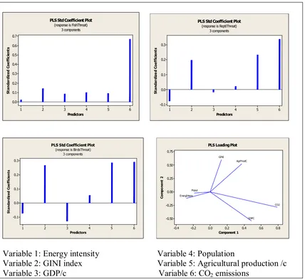
[image:21.595.86.513.599.727.2]The graphs in Figure 3 show the effect of each independent variable on the
dependent variable. Specifically the graph on the top left corner shows that all the
explanatory variables have a positive influence on the dependent variable fish in
threat with the variable CO2 emissions to have the most significant effect, with the
variable income inequality to follow and the variable energy intensity to have the
[image:22.595.86.514.276.668.2]lowest effect.
Figure 3: Individual effects of independent variables on the dependent variable
6 5 4 3 2 1 0.7 0.6 0.5 0.4 0.3 0.2 0.1 0.0 Predictors St an da rd iz ed C oe ff ic ie nt s
PLS Std Coefficient Plot (response is FishThreat)
3 components 6 5 4 3 2 1 0.3 0.2 0.1 0.0 -0.1 Predictors St an da rd iz e d Co ef fic ie nt s
PLS Std Coefficient Plot (response is ReptiThreat)
3 components 6 5 4 3 2 1 0.3 0.2 0.1 0.0 -0.1 Predictors S ta n da rd iz ed C oe ff ic ie n ts
PLS Std Coefficient Plot (response is BirdsThreat)
3 components
-0.4 -0.2 0.0 0.2 0.4 0.6 0.8
0.75 0.50 0.25 0.00 -0.25 -0.50 Component 1 Co m po ne nt 2 CO2 AgrProdC Popul GDPC GINI EnergIntens
PLS Loading Plot
Variable 1: Energy intensity Variable 4: Population
Variable 2: GINI index Variable 5: Agricultural production /c Variable 3: GDP/c Variable 6: CO2 emissions
Similarly the graph on the top right corner and in the case of reptiles in threat
the variables energy intensity and GDP/c have a very low negative influence. On the
as expressed by the GINI index have significant positive influence while population
has a small positive effect.
The graph on the bottom left corner refers to the birds endangered and shows
the same picture as in the case of birds but with higher negative effects for the
variables energy intensity and GDP/c and almost equal positive influence for the
variables income inequality, agricultural production and CO2 emissions.
Finally in the graph on the bottom right corner we can see that the variables
population and energy intensity have the smallest effect compared to the other
variables.
6. Conclusions and policy implications
Relying on a sample of 71 countries and a number of economic and
environmental variables we modelled and interpreted functionally the protection of
various species in threat like reptiles, mammals, fish, birds, trees and plants. Due to
the high asymmetric distribution of the dependent variables the mean regression
cannot capture adequately the dimension of the species in threat. Comparing to the
parametric estimates lead us to conclude that in such cases there exists a nonlinear
relationship. The quantile regression is more preferable to the linear one as it enables
us to look at the changes in the dependent variable in reaction to changes in the
independent variables at different points of the distribution.
Specifically, as explained the quantile regression refers not to the mean
influence of the independent variables on the mean value of the dependent variable
but on a number of different quantiles. It also seems that explanatory variables have a
substantial influence on species in threat either at the bottom or at the top of the
agricultural production (with an exception in the 70th quantile) and income inequality
increases as we move from the 10th to the 90th quantile. On the contrary a stable
influence can be observed for CO2 emissions and population as we move along the
quantiles. A mixture of changes is observed in the case of mammals in threat.
We have found that in the cases of the GINI index OLS overestimates the
estimated parameters till the 70th quantile and then underestimates parameters while
for the agricultural production underestimation takes place till the upper quantilies
(80th). In the cases of population and CO
2 OLS first underestimates (till the 35th) then
overestimates (till the 80th) and then it underestimates again the estimated coefficients.
For the constant term there is a complete underestimation.
On the other hand, all the explanatory variables have a positive effect in the
case of fish in threat with the variable emissions to have the most significant
influence, the income inequality the second significant effect and the energy intensity
the lowest power. In the case of reptiles endangered the variables energy intensity and
GDP/c have a low negative effect. On the contrary, the variables emissions, income
inequality and agricultural production have the most significant positive influence and
the population to have a low positive effect. In terms of income inequality our results
come in line and extend those of Mikkelson et al. (2007). Finally, the threatened birds
show the same picture as the reptiles but with higher negative effects for the variables
energy intensity and GDP/c and almost equal influence in the case of income
inequality, agricultural production and emissions. It worth mentioning that population
and energy intensity variables have the lowest effect compared to the others.
The policy implications are interesting. The vast population increase,
urbanisation and extension of economic activities make the preservation of natural
limited capital for the environment and facing the great threat of extinction of some
species, the decision makers have to put priorities making sure that the efforts of
preserving biodiversity move to the right directions.
Quantile regression can be used effectively by ecologists. Due to complex
interactions among organisms statistical distributions of ecological data have usually
unequal variation. These interactions are not easily taken into consideration by
statistical models. At the same time this unequal variation implies that there is not
only a single rate of change (slope) that describes the relationship between a
dependent and an explanatory variable measured on a subset of these factors. A
solution to this limitation is the quantile regression, which estimates multiple slopes
from the minimum to the maximum response and allows for a full picture of the
relationships between response variable and regressors (Cade and Noon, 2003).
These slopes cannot be equal for all quantilies in cases where we have
heterogeneous error distributions. This is the case in our analysis but it is expected to
be the case in a range of ecological applications. Specifically complex forms of
heterogeneous response distributions are expected in cases where important processes
are not included in the model. In such cases we expect rates of changes of greater
magnitude in the extreme quantiles (<30% or >70%) compared to the central
estimates (50%). Using quantile regressions in models with unequal variances allow
us to explore the associated effects with variables that may have been omitted as
statistically insignificant on mean estimates. Our task is to tackle the large variation
usually met in cases of detecting the relationship between ecological variables and the
hypothesised casual factors not ascribed to random sampling variation.
The valuation of ecosystem services requires the integration of ecological
economists (Perrings and Walker, 1995). A number of actions with the formation of
national policy for the preservation of every country’s biodiversity, the establishment
and operation of protected areas, the effective protection of species in threat, the
conservation of genetic material of endemic plants and animals and the sensitiveness
and the notification of the problem to all citizens and countries.
Biodiversity does not remain stable and for this reason a simple enumeration
and recording is not sufficient. At the same time the scale of locality together with the
global dimension of the problem make the formation of adequate policies difficult.
This implies that the decision maker must take into consideration both the local and
the national (global) scale and dimension of the problem in scheduling policies for the
References
Brody, S.D. (2003). Examining the Effects of Biodiversity on the Ability of Local Plans to Manage Ecological Systems. Journal of Environmental Planning and Management, 46(6), 817 – 837.
Buchinsky, M. (1995). Estimating the asymptotic covariance matrix for quantile regression models: A Monte Carlo study. Journal of Econometrics, 68, 303-338.
Buchinsky, M. (1998). Recent advances in quantile regression models. Journal of Human Resources 33(1): 88-126.
Cade, B.S., Terrell J.W. & Schroeder R.L. (1999). Estimating effects of limiting factors with regression quantile. Ecology80: 311-323.
Cade, B.S. & Noon B.R. (2003). A gentle introduction to quantile regression for ecologists
.
Frontiers in Ecology and the Environment, 1(8): 412-420.Clausen, R. & York, R. (2008). Global biodiversity decline of marine and freshwater fish: A cross-national analysis of economic, demographic and ecological influences.
Social Science Research, 37, 1310-1320.
Costanza, R., Fisher, B., Mulder, K., Liu, S. & Cristopher, T. (2007). Biodiversity and ecosystem services: A multi scale empirical study of the relationship between species richness and net primary production. Ecological Economics, 61, 478-491.
Delong, B. (2003). Estimating world GDP, one million B.C.-present. Department of Economics, University of California, Berkley.
Dietz, S. & Adger W.N. (2003). Economic growth, biodiversity loss and conservation effort. Journal of Environmental Management, 68, 23-35.
Faith D.P. (2002). Quantifying biodiversity: a phylogenetic perspective. Conservation Biology, 16(1): 248-252.
Groeneveld, R., Grashof-Bokdam, C. & van Ierland, E. (2005). Metapopulations in Agricultural Landscapes: A Spatially Explicit Trade-off Analysis. Journal of Environmental Planning and Management, 48(4), 527 – 547.
Halkos, G.E., 2003. Environmental Kuznets Curve for sulfur: evidence using GMM estimation and random coefficient panel data models. Environment and Development Economics, 8(04), 581-601.
Hoffman, J. (2004). Social and environmental influences on endangered species: a cross-national study. Sociological Perspectives, 47(1), 79-107.
Hui, D., Biggs, R., Scholes, R.J., Jackson R.B. (2008). Measuring uncertainty in estimates of biodiversity loss: The example of biodiversity intactness variance
Hughes, J. B., Daily, G. C., & Ehrlich, P. R. (1997). Population diversity: Its extent and extinction. Science, 278, 689–692.
Jones, M.C. (1992). Estimeting densities, quantiles, quantiles densities and density quantiles. Annals of the Institute of Statistical Mathematics, 44(4), 721-727.
Koenker, R., Bassett Jr, G. (1978). Regression quantiles. Econometrica, 46(1), 33-50.
Koenker, R., Bassett Jr, G. (1982). Robust tests for heteroskedasticity based on regression quantiles. Econometrica, 50(1), 43-62.
Koenker, R. (2005). Quantile regression. New York: Cambridge University Press.
Mikkelson G.M., Gonzalez A. and Peterson G.D. (2007). Economic Inequality Predicts Biodiversity Loss. PLoS ONE, 5, e444.
Naidoo, R., Adamowicz, W. (2001). Effects of economic prosperity on numbers of threatened species. Conservation Biology, 15(4), 1021-1029.
Newey, W.K., Powell, J.L. (1987). Asymmetric least squares estimation.
Econometrica, 55(4), 819-847.
Noss R.F. (1990). Indicators for monitoring biodiversity: a hierarchical approach.
Conservation Biology, 4,355.
Nunes, P.A.L.D. & van den Bergh, J.C.J.M. (2001). Economic valuation of biodiversity: sense or nonsense? Ecological Economics, 39, 203-222.
O' Connor C., Marvier M. & Kareiva P. (2003). Biological vs. social, economic and political priority-setting in conservation. Ecology Letters6: 706-711
Perrings, C., Mäler, K.-G., Folke, C., Hollings, C.S., Jansson, B.-O. (1995). “Introduction: framing the problem of biodiversity loss”. In: Perrings, C., Mäler, K.-G., Folke, C., Holling, C.S., Jansson, B.-O. (Eds.), Biodiversity Loss: Economic and Ecological Issues. Cambridge Univ. Press, Cambridge, UK, pp. 1–17.
Perrings, C., Walker, B. (1995). “Biodiversity loss and the economics of discontinuous change in semiarid rangelands”. In: Perrings, C., Mäler, K.-G., Folke, C., Holling, C.S., Jansson, B.-O. (Eds.), Biodiversity Loss: Economic and Ecological Issues. Cambridge Univ. Press, Cambridge, UK, pp. 190–210.
Powell, J. (1986). Censored regression quantiles. Journal of Econometrics, 32, 143-155.
Scholes R.J. & Biggs R. (2005). A biodiversity intactness index. Nature434(3): 248-252
Terrell J.W., Cade B.S., Carpenter J. & Thompson J.M. (1996). Modelling stream fish habitat limitations from wedged–shaped patters of variation in standing stock.
Transactions of the American Fisheries Society, 125,104-117.
Turner, R.K., Button, K. & Nijkamp, P., (Eds) (1999). Ecosystems and Nature: Economics, Science and Policy. Elgar, Cheltehham.
United Nations Development Programme (2000). United Nations Environment Programme, World Bank, World Resources Institute (WRI). World Resources 2000-2001. Elsevier, Amsterdam.