Learning by exporting in Turkey: an investigation for existence and channels

(1)

Munich Personal RePEc Archive

Learning by exporting in Turkey: an

investigation for existence and channels

Maggioni, Daniela

3 January 2010

Online at

https://mpra.ub.uni-muenchen.de/37157/

(2)

Learning by exporting in Turkey: an

investigation for existence and channels

∗

Daniela Maggioni

†

Universit`a Politecnica delle Marche

Abstract

Using a rich longitudinal database at the plant level, I shed new light on the causal nexus between exports and productivity for Turkey, a middle-income country. I find evidence for both self-selection into exporting and learning-by-exporting. My main focus is on post-entry effects. To test this hypothesis I follow recent empirical literature and I apply the Propensity Score Matching and a Difference-in-Difference estimator. I find a higher la-bour productivity and TFP growth for exporting firms in the entry year and some years following the entry. Exports seem to place firms on a super-ior productivity path. My main contribution is to show the strict linkage between export and import activity: export starters often start also im-porting. Learning by exporting effects hold when I control for the role of imports and I verify larger productivity gains for firms which start exporting and importing at the same time. Finally, in order to verify if post-entry ef-fects are not only scale efef-fects but work through competition channel and/or technology transfers, I look for a heterogeneity according to the sectoral productivity gap between the domestic market and foreign trade partners. I verify a different timing of efficiency improvements between comparative advantage and disadvantage sectors.

Keywords: Exports, Self selection, Learning-by-exporting, Imports JEL codes: F14, D24

∗_{I wish to thank Prof. Giuliano Conti for useful comments and financial support,}

and Prof. Erol Taymaz for discussions and suggestions. I’m grateful to the Turkish State Institute of Statistics (TURKSTAT) for providing access to firm level data under a confidential agreement. In particular, I thank Ferhunde Demirbag, Nilgun Dorsan, Kenan Orhan, Oguzhan Turkoglu and Erdal Yildirim from Turkstat. Valentina Adorno, Carlo Altomonte, Alessia LoTurco, Anna Maria Falzoni, Ana Maria Fernandes, Seda Koymen, Chiara Tomasi, seminar and conference participants at the Bilkent University, ITSG 2009, SSES 2009 and ETSG 2009 provided valuable comments. The usual disclaimers apply.

†_{Universit`a Politecnica delle Marche, Department of Economics, Piazzale Martelli 8,}

(3)

1 Motivation and previous literature

The nexus between trade and economic growth has always drawn the at-tention of economists and, traditionally, the research on this topic has been conducted at a macro level - country or industry level. The recent availability of firm and plant level datasets and the following proliferation of firm-level analysis has shown new stylized facts, especially the co-existence in the same sector of firms with heterogeneous characteristics, and has renewed the in-terest for the link between exports and efficiency/productivity.

Theoretical and empirical literature has verified, both for developed and developing countries, a superior performance of firms involved in interna-tional markets (Bernard and Jensen, 1999; Bernard et al., 2003; Clerides et al., 1998; Pavcnik, 2002). Since the finding of this evidence, a large number of studies have investigated, in more detail, the causal relationship between exports and firm productivity. Two main hypothesis have been suggested. First, there exist additional costs of selling goods in foreign markets: trans-portation costs, distribution or marketing costs, and costs in adapting do-mestic products to foreign consumers’ tastes. These costs represent an entry barrier and one may expect more productive firms to self-select into export markets because they are more likely to cope with these sunk costs and sur-vive in the international market. This is the first suggested hypothesis. The self-selection mechanism has also been sustained by new heterogeneous firms’ models (Melitz, 2003; Bernard et al., 2003) that hypothesize the differential of productivity between firms pre-exists1_.

The second hypothesis behind the positive correlation between firm trade and efficiency concerns the role of learning-by-exporting. Previous empirical literature has suggested three main channels through which exports may increase firms’ productivity: technology adoption, the exploitation of scale economies and a higher competitive pressure2_.

While there is large consensus on the self-selection hypothesis (for ex-ample, Bernard and Jensen, 1999; Clerides et al., 1998; Aw et al., 2000; Delgado et al. 2002), there is less empirical evidence supporting learning-by-exporting, results are often controversial and also channels through which

1

Recently, some scholars have also hypothesized a conscious self-selection, supposing the existence of a forward-looking behaviour. See, for example, Alvarez and Lopez, 2005.

2_{First, exporting firms may increase their knowledge through the access to new}

(4)

learning could display are not clear. Wagner (2007a) review 54 micro-econometric studies with data from 34 countries, confirming that exporters are more pro-ductive than non-exporters, and the more efficient firms self-select into export markets. Post-entry effects are usually negligible or lacking, and learning-by-exporting hypothesis fails for developed and competitive countries (see for example Wagner, 2007b, who analyses West German plants). In high-income countries firms are already on the technological frontier, they are operating in an efficient and competitive context and they are using advanced technology. There could be no great learning effects in such a framework. In oppos-ite, in a developing country, firms could take advantage of export activity through technology transfers and contacts with more efficient foreign firms, especially if they enter a developed and competitive foreign market. Kraay (1999) for China, Blalock and Jertler (2004) for Indonesia, Van Biesebroeck (2003) for Cote d’Ivoire, Fernandes and Isgut (2007) for Colombia and De Loecker (2007) for Slovenia find some positive productivity effects stemming from export entry3_.

I join this debate and present empirical evidence on the relationship between exports and firm performance for Turkey in the period 1990-2001. Turkey is an interesting country to analyse because it is a middle-low in-come country which underwent, during the ’80s, a process of trade open-ness4_{. Its main trade partners are advanced countries}5_{, and, in opposite}

to less developed economies, its firms may be endowed of the human cap-ital and capabilities to absorb positive spillovers and exploit opportunities granted by international markets. All these features make Turkey an ideal context where learning-by-exporting effects could display and be the outcome of technology/knowledge transfers and a more competitive environment, and not only caused by economies of scale.

I study both the directions of causality between exports and productivity, even if I especially focus on the learning-by-exporting hypothesis that has stronger policy implications for export promotion6_.

Previous empirical evidence for Turkey on this topic is based mainly on

3_{Castellani (2002) and Serti and Tomasi (2008) have displayed a potential for}

learning-by-exporting for Italy. Even if Italy is a developed country, it is not on the technological frontier in many (especially high-technology) manufacturing sectors, its productive system is less competitive than other European countries, its main trade partners, and there could be some scope for positive effects from export activity.

4_{During the ‘80s it moved from an import substitution regime to the implementation}

of export-promotion policies.

5

More than 80% of its exports are directed to OECD countries.

6

(5)

two studies. Yasar and Rejesus (2005)7_{, applying Propensity Score Matching}

(PSM) techniques and Difference-In-Difference (DID) estimators, show that learning-by-exporting may be the reason for the positive correlation between exporting status and firm performance. They find out a productivity differ-ential in the entry year and two years after entry8_{, but their analysis concerns}

only a small sample of sectors. Aldan and Gunay (2008), using a different database (from Central Bank of the Republic of Turkey) and same economet-ric approach, highlight that both self-selection and learning-by-exporting are important. Their analysis supports positive post-entry effects on firm labour productivity and employment.

With this paper I confirm previous findings extending the analysis, com-pared to Yasar and Rejesus, to a large dataset, including all manufacturing sectors, and a wider time horizon. In opposite to Aldan and Gunay who analyse labour productivity, I focus on TFP and I also investigate other im-portant firm characteristics. My contribution is also to show the link between the export entry and import activity at firm level, two forms of international involvement that are strictly related. Previous literature has disregarded this relationship9_{, and I try to fill this gap.}

Then, I add some evidence on the channels of learning-by-exporting, look-ing for an heterogeneity in post-entry effects accordlook-ing to the type of sector. Previous papers usually do not pay attention on the reasons and motivations behind post-entry effects. The only two exceptions are Fernandes and Isgut (2007) and De Loecker (2007) who verify a significant and larger positive advantage of participation in export market for plants selling a great share of their exports to high-income countries. This evidence sheds some light on the channels of the learning: if there are different effects according to trade partners, it is likely exporting effects work also through competition channel and technology transfers and not only through a scale effect. Behind their approach there is the idea that firms of every sector can learn when they enter advanced countries. My idea is that the important feature is not only the technological level or efficiency of destination country, but the gap between the destination country and the domestic market. I investigate if the

7_{They use data, like my dataset, from Turkstat but they analyse a smaller sample}

(three four-digit sectors) for a restricted time period 1990-96.

8

Yasar and Rejesus (2005) examine effects of both the entrance and exit behaviour of plants.

9

(6)

potential for learning is higher in sectors more distant to the technological frontier10 _{because in these sectors spillovers may be more important.}

The next section gives a brief description of data and verifies for Turkey the existence of the “Exceptional exporters’ performance”. Sections 3 and 4 present results on self-selection and learning-by-exporting hypothesis. In Section 5 I go in search of learning channels, I analyse the link between export entry and import activity and I try to characterise sectoral post-entry effects according to comparative advantage. A final Section gives concluding remarks.

2 Data and descriptive analysis

2.1 Data

In this paper I use an original Turkish plant-level database11_{, from the Annual}

Surveys of Manufacturing Industries, collected by Turkish State Institute of Statistics (Turkstat). I have at my disposal an unbalanced panel dataset on plants with more than 25 employees for the whole manufacturing sector in the period 1990/200112_{. The dataset consists of plant-level information}

on output, inputs, investments13 _{and a large number of plant characteristics}

(foreign ownership, import activity, export activity, size, industry, region). All nominal values are deflated using 4-digit ISIC price indices (the base year is 1994) provided by Turkstat, while for capital goods I use a unique deflator for all sectors, but different deflators according to type of goods (machinery and transportation). After a cleaning procedure14, I remain with a dataset

10_{As an indicator of distance to technological frontier I use a sectoral indicator of revealed}

comparative advantage. See the following analysis for an explanation of this approach.

11_{The observation unit is a plant that has its own accounts. I use the terms firm and}

plant as synonym because most of the firms are single plant firms.

12

Turkstat collects data on plants with more than 10 employees, but before 1992 it ran two different surveys for firms with more 25 employees and firms with less than 25 employees. In order to keep a longer time horizon as possible I have decided to use data for larger firms. In addition, I am interested in export activity and only few firms with less 25 employees export, and, anyway, their export volume is very low.

Import and export data at plant-level are from Foreign Trade Statistics.

13_{I have used the Perpetual inventory method in order to obtain a capital stock measure.} 14_{I drop observations with missing data for variables of interest (output, input variables),}

(7)

of 5,783 firms, for a total of 46,607 observations. There are 3,072 firms ex-porting at least in one year in the period 1990/2001 (in opposite 2,711 firms never export). I use, as performance indicator, both labour productivity and TFP indicators. I calculate labour productivity as value added per employee. TFP measure is estimated using the semiparametric approach by Levinshon and Petrin (2003) and I have estimated the production function separately for every 2-digit (ISIC) sector (T F P). I have also applied the semiparametric approach taking into account the export status of firms (T F Pexp)15_{. Finally,}

as my robustness check, I have constructed a multilateral TFP index follow-ing Good et al. (1997), T F Pindex_.

2.2 Exceptional exporters’ performance

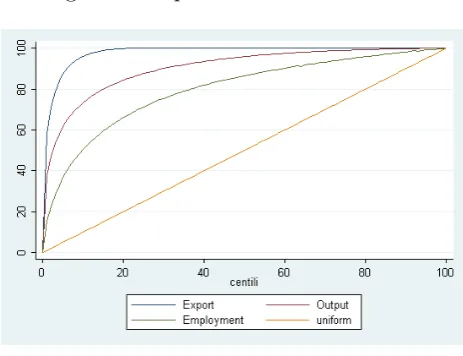
[image:7.595.180.412.448.626.2]

Figure 1 shows that in Turkey exports are highly concentrated, more than output and employment, in few large exporters as documented also for other European countries (Mayer and Ottaviano, 2007). This means that, if there are significant post-entry effects, export activity is positively affecting only a part of firms’ population16_.

Figure 1: Export Concentration 2001

sample less than three years.

15_{I have modified the Levinshon and Petrin (2003) procedure in order to take into}

account the export status as an additional control in the dynamic problem (see Van Biesebroeck, 2005 and De Loecker, 2007).

16_{The beneficial impact of trade could be concerning a still smaller population if}

(8)

Table 1 gives an overview of the firm international involvement in my database. During the analysed period (1990/2001), the share of exporters in the sample is quite constant (about 25/32%). Even if in 1996 the Cus-toms Union agreement with the European Union (EU) went into effect, EU had already removed tariffs on imports from Turkey before 199617_{. A large}

[image:8.595.141.450.274.453.2]

number of exporters are involved also in import activity: more than 65% of exporters are two-way traders.

Table 1: Firms in international trade

Y ear Exporters Only Exporters Only Importers T woW ay T raders

(%) (%) (%) (%)

1990 25.35 8.68 10.74 16.67 1991 29.80 11.22 12.06 18.58 1992 28.63 11.45 11.74 17.18 1993 28.42 10.23 11.21 18.19 1994 30.55 11.48 10.05 19.08 1995 32.20 11.99 10.39 20.21 1996 26.34 8.36 11.49 17.98 1997 25.51 6.80 11.40 18.71 1998 28.84 8.83 12.50 20.01 1999 27.93 8.48 12.92 19.45 2000 30.13 10.54 13.16 19.59 2001 31.17 10.56 13.22 20.61

My elaborations from firm level dataset.

Simple descriptive statistics (Table 2) confirms, also for Turkey, the “ex-ceptional exporters’ performance”: exporters present a significant higher pro-ductivity (TFP and labour propro-ductivity)18_{, they have a larger number of}

em-ployees and a larger output, they are more capital intensive, and it is more likely they are importers and foreign-owned.

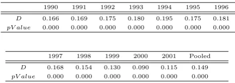
This table displays differences just in the mean value. A test for stochastic dominance, the Kolmogorov-Smirnov test, also allows to consider all mo-ments of the productivity distribution for exporters and non-exporters19_.

The test displays, both for each year in the sample and for the whole period (pooled sample), that TFP distribution of exporters stochastically dominates

17_{Customs Union had more effects on the tariffs on Turkish imports, so the impact of}

this agreement was mainly on Turkish import flows.

18_{The export advantage in productivity concerns all industries and all dimensional}

classes. Relative data are available upon request.

19

(9)

Table 2: Descriptive Statistics

T F P LP K/L Size F DI Import

Exporter 40.11 719.74 588.57 246 8.85 65.83

N onExporter 29.97 483.86 370.11 114 3.82 16.46 All differences are statistically significant at 1%

[image:9.595.178.415.311.395.2]

that of non-exporters20_.

Table 3: Kolmogorov Smirnov test. TFP

1990 1991 1992 1993 1994 1995 1996

D 0.166 0.169 0.175 0.180 0.195 0.175 0.181

pV alue 0.000 0.000 0.000 0.000 0.000 0.000 0.000

1997 1998 1999 2000 2001 Pooled

D 0.168 0.154 0.130 0.090 0.115 0.149

pV alue 0.000 0.000 0.000 0.000 0.000 0.000

HA: Exporters stochastically dominate Non Exporters. Test on logarithmic TFP.

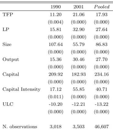
In order to strengthen this descriptive evidence, I follow Bernard and Jensen (1999) and check for other firm characteristics: firm size, industry and regional localisation. Table 4 shows the β coefficient of the following OLS regressions21_:

yit =α+βexport dummyit+δsizeit+dj +dt+dr+ǫit (1)

where y can be: TFP, labour productivity, capital stock, capital intensity (the ratio between capital stock and number of employees), number of employees (as a proxy for firm size), output and unit labour cost (calculated as total labour cost on output). The variable export dummyit indicates the export

status of the firm in the period t. dj, dt and dr are sectoral, time and

regional dummies. All coefficients are statistically significant. Even if I check for additional controls (firm size, industry, region, year), the superior performance of exporters holds. I display an export premium of 18% for TFP

20_{I do not show the graphical analysis that is available upon request.} 21

(10)

[image:10.595.205.391.201.415.2]

in the pooled sample. This evidence for Turkey is consistent to findings for other countries22_.

Table 4: Export Premium

1990 2001 P ooled

TFP 11.20 21.06 17.93 (0.004) (0.000) (0.000) LP 15.81 32.90 27.64

(0.000) (0.000) (0.000) Size 107.64 55.79 86.83

(0.000) (0.000) (0.000) Output 15.36 30.46 27.70

(0.000) (0.000) (0.000) Capital 209.92 182.93 234.16 (0.000) (0.000) (0.000) Capital Intensity 17.12 55.85 40.71

(0.011) (0.000) (0.000) ULC -10.20 -12.21 -13.22

(0.000) (0.000) (0.000)

N. observations 3,018 3,503 46,607 Robust standard errors are calculated. P-Values are in brackets. Coefficients have been transformed in exact percentage values as (expβ₋₁₎_∗_100.

Coefficients are from regressions controlling for sector, region and time dummies and for the firm size.

3 Self Selection

In the previous section, I have verified the positive correlation between ex-port and some firm performance indicators. Now, being interested in shed-ding light on the causal relationship, I keep in my dataset firms that start exporting in the sample period and firms which never export.

I define export starter as a firm which continuously exports from t onwards (for at least two consecutive years) and which had never exported in the previous years (I request to observe at least t-1 and t-2)23_{. I end up with 8} 22_{For example De Loecker (2007) finds out a labour productivity premium of 30%; Serti}

and Tomasi (2008), for Italy, show a TFP premium between 7.5% and 15% according to the year of analysis.

23_{I allow exporters to exit the export market only one year. If starters stop exporting}

(11)

cohorts, one for each years between 1992-99, and 543 starters24_.

I analyse ex-ante differences between starters and never exporters in order to investigate the self-selection hypothesis. Following Bernard and Jensen (1999), I regress the productivity indicators and other firm characteristics (all in logarithm, with the exception of skill ratio and import share) in the pre-export time t −σ (1 ≤ σ ≤ 525_{) on a dummy indicating if a firm is}

an export starter at time t, starti,t, and on a set of controls (number of

employees, sectoral dummies, regional dummies and time dummies):

yi,t−σ =α+βstarti,t+δsizei,t−σ +ηdj +ωdt−σ +µdr+ǫit (2)

whereyi,t−σ is firm-level variables in level or growth rate.

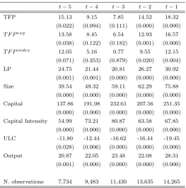
When I investigate variables in levels (Table 5) the empirical evidence sup-ports the self-selection hypothesis: more productive firms become exporters. This is confirmed both when I use labour productivity and total factor pro-ductivity (TFP index or TFP from Levinshon and Petrin estimation). Before entering export market starters are more productive, larger, present higher capital intensity and higher output than never exporters. These differences are persistent and are at work for the whole pre-entry period, with the ex-ception of TFP, for which there are pre-entry premia in t-1, t-2 and also t-5. One can especially notice a huge advantage for starters in capital and size.

Also, I verify whether firms modify their behaviour in the pre-entry period according to the future export status analysing the growth rates. I find out that future exporters increase their size, their market share and, even if for only one year (t-2), their productivity (the relative table is available upon request), but one can not affirm that these changes are in preparation to export entry, having in mind the international market, or if these changes allow firms to enter the export market in the following period. Looking at the whole pre-entry period it is highly likely that future starters are successful firms, also before exporting, and they can enter export market because of their pre-export performance.

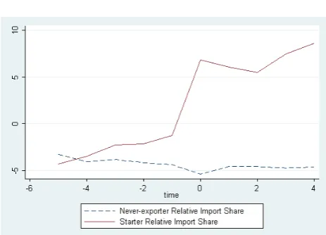
In the pre-entry period an interesting evidence is detected for import par-ticipation. Import and export activities are strictly linked and the Figure 2 shows an increasing import share gap between never exporters and starters26_.

In particular, one can notice a significant jump between t-1 and t (for firms that never export throughout the sample period t=0 is just the median year in the sample, so 1995): some firms entering export market also start im-porting materials at the same time. Different explanations for this finding

24_{The distribution of starters across the cohorts is available from author upon request.} 25_{As in Serti and Tomasi (2008)}

26

(12)

[image:12.595.165.429.158.425.2]

Table 5: Self-Selection: Levels

t−5 t−4 t−3 t−2 t−1 TFP 15.13 9.15 7.85 14.52 18.32 (0.022) (0.094) (0.111) (0.000) (0.000)

T F Pexp _13.58 _8.45 _6.54 _12.93 _16.57

(0.038) (0.122) (0.182) (0.001) (0.000)

T F Pindex _12.05 _5.16 _0.77 _9.55 _12.15

(0.071) (0.353) (0.879) (0.020) (0.004) LP 24.75 21.44 20.81 26.27 30.92

(0.001) (0.001) (0.000) (0.000) (0.000) Size 39.54 49.32 59.11 62.29 75.88

(0.000) (0.000) (0.000) (0.000) (0.000) Capital 137.86 191.98 232.61 207.56 251.35 (0.000) (0.000) (0.000) (0.000) (0.000) Capital Intensity 54.99 73.21 80.87 63.58 67.85

(0.000) (0.000) (0.000) (0.000) (0.000) ULC -11.80 -12.44 -16.62 -16.44 -19.45

(0.028) (0.006) (0.000) (0.000) (0.000) Output 20.87 22.05 23.48 22.08 28.31

(0.001) (0.000) (0.000) (0.000) (0.000)

N. observations 7,734 9,483 11,430 13,635 14,265

Robust standard errors are calculated. P-Values are in brackets. Coefficients are from regressions con-trolling for sector, region and time dummies. The employment and capital regressions do not include the size as control variable.

Note: TFP is the total factor productivity calculated from Levinshon and Petrin (LP) approach.T F Pexp

is the productivity indicator from LP approach and taking into account the export status. T F Pindex _is

the multilateral TFP index following Good et al. (1997).

could be suggested. These two international activities may share the same sunk costs, and when firms start being involved in international markets, through imports or exports, they take part of some networks with foreign firms which may ease other internationalisation strategies. Import activity may help firms to set up relationships with local operators and understand and know the foreign markets. This experience could facilitate the export activity. In addition, the use of imported inputs may allow firms to pro-duce and adapt goods meeting the preferences, habits and tastes of foreign consumers27_{. Finally, foreign sourcing of cheaper and/or high quality inputs}

could lead to productivity and efficiency improvements for firms that become able to penetrate foreign markets28_.

27

This could especially be important for firms in developing countries exporting to ad-vanced economies

(13)

[image:13.595.180.412.295.462.2]

Even if it is difficult to clean the export effect from a potential import effect, it is important to have in mind in the following analysis that a great part of export starters are also involved in import activity and this for-eign sourcing may start in conjunction with export entry. Previous papers, studying the link between exports and productivity, sometimes investigate the foreign/domestic ownership of starters and never exporters but they do not take into account if a firm is also an importer, and up to now literature has neglected the relationship between exports and imports at firm-level in the learning-by-exporting investigation29_.

Figure 2: Import Share Trend

4 Post-Entry Effects

According to the previous investigation, a self-selection mechanism drives the most successful, large and efficient firms in the export market. Self-selection does not exclude the potential for learning by exporting. Even if starters are already more productive when they enter foreign markets, they could further improve their performance and the differential with non exporters after the export entry. In order to test this hypothesis I consider a treatment model, where treatment is the export entry. Treated units are export starters,

positive correlation may simply mean that the same firms that can cope with sunk export entry costs are also able to set relationships with foreign suppliers.

29_{Kasahara and Rodrigue (2008) look at the opposite direction controlling for export}

(14)

and controls are never exporting firms in the sample. Treatment does not concern only one specific year, but for every starter cohort there is a different treatment year. I am interested in the average treatment effect on the treated (ATT),

AT T = E(Yit(1)−Yit(0)|Di = 1) =

= E(Yit(1)|Di = 1)−E(Yit(0)|Di = 1) (3)

that is the difference for a treated firm between the outcome it obtains after exporting and the potential outcome it would have obtained if it had never exported. I am verifying if, in the hypothetical counterfactual situation of no exporting, starters would have had worse or better outcomes. I am not able to observe both outcomes for the same firm, especiallyE(Yit(0)|Di = 1)

- that is the outcome of exporters if they had not exported - is unknown. I can only calculate E(Yit(0)|Di = 0), the outcome for non exporters provided

that they have not exported. This means that there could be a selection bias concerning the computation of ATT that can be written as:

B(AT Tt) =E(Yit(0)|Di = 1)−E(Yit(0)|Di = 0) (4)

If the group of the treated is randomly selected from the population, that means the treated and the control group have the same observable and non-observable characteristics, the bias will be zero. The problem is that selection into treatment is not random and treated and non-treated firms may differ in important characteristics. I have already verified the exist-ence of these differexist-ences in the previous self-selection analysis: self-selection bias is a real problem. Using a generic non exporter will not allow me to make causal inferences because pre-entry differences in firm characteristics may explain the difference in post-entry productivity levels of exporters and non-exporters. To solve this problem, I use both Propensity Score Matching (PSM) and Difference-In-Difference (DID) strategy30. With matching tech-niques I can construct a consistent counterfactual. In this way, if difference in productivity remains, it can be attributed to firm export activity rather than other characteristics; in opposite if there is no difference one can think that exporting does not benefit firms.

The basic idea of matching is to find, in a large group31 of non treated units (never exporters), those firms who are similar to the starters in all

30_{As affirmed by Blundell and Costa Dias (2000) the use of matching estimator in}

combination with DID approach can “improve the quality of non-experimental evaluation results significantly”.

31

(15)

relevant pre-treatment (observable) characteristics to approximate the coun-terfactual outcome (Blundell and Costa Dias, 2000).

The PSM consists in estimating a propensity score of export entry condi-tional to variables at my disposal and that, in my beliefs, could affect the probability to enter export market. Then, I match treated plants with con-trol plants using this estimated propensity score. I use the following probit to estimate the probability score of first-time exporting32_:

P r(ST ARTit= 1) =f{T F Pt−1, nt−1, kt−1, ulct−1, SkillP rodt−1, Importt−1,

F oreignSharet−1, SubInpt−1, SubOutt−1, dummies}

(5)

where ST ARTit is a dummy variable assuming value 1 if the firm starts

exporting in t. The chosen probit specification satisfies the balancing test introduced by Rosenbaum and Rubin (1983) and formalized in Becker and Ichino (2002)33_{. This probit is estimated pooling all cohorts}34_{. In the}

regres-sion I have kept only never exporters, for all the years they are in the sample, and starters, for the year they start exporting. I include the following vari-ables lagged one year35_{: total factor productivity, size, the square of the size,}

capital stock, unit labour cost, the share of skilled production employees, foreign share36_{, import status, subcontracted input and output shares, and}

dummies for industry, year and region. The probit specification I choose per-mits to correctly classify 95.58% of observations. Using the estimated scores I match plants applying the “Nearest Neighbor” (NN) matching on the “com-mon support”37_{. The NN technique matches a starter with a never exporter} 32_{As robustness checks, I have also tried to use other probit specifications, always}

satis-fying the balancing test (Rosenbaum and Rubin, 1983). Basic results for following analysis are quite similar using these specifications.

33_{The matching of plants is “balanced” if observations with the same propensity score}

have the same distribution of observable (and unobservable) characteristics regardless of treatment status. This test tells that the decision to export is random, treated and control units are identical on average.

34

I have decided to use the pooled sample because, in this way, I can exploit the inform-ation contained in the largest possible dataset for modeling the export-starting decision. Estimating different probit for each cohort could lead to a loss of efficiency because the number of starters in every cohorts is low.

35_{I include lagged variables because the observable covariates I use to estimate the}

propensity score should not be affected by treatment. This means that also variables that are affected by the anticipation of the export entry should not be included in the model. Anyway it is difficult to be sure that firms do not change some important characteristics in preparation to export entry.

36_{The capital share owned by foreign shareholders.}

37_{I have chosen to match the starter with a single never exporters because of the large}

(16)

having the closest propensity score and I also allow that never exporters are used as a match more than once - matching “with replacement”.

I have followed Girma et al. (2003) and I have applied matching cross-section by cross-cross-section (separately for each cohort). I restrict, in this way, the matches to come from the same year. Because I do not restrict matches to come also from the same sector38_{, I have calculated ATT effects both on}

absolute and relative variables (in the latter case, variables are expressed as a deviation from the industry-year mean, in order to take into account the sectoral and time evolution). I have also applied the matching to the pooled sample, that means a starter could be matched with a never exporter who has the most similar propensity score, but it could be from a different year and a different sector39_{. Results obtained from the matching implemented}

cross-section by cross-section and the matching implemented on the pooled sample are very similar.

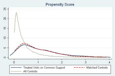
Since I do not condition on all covariates but on the propensity score, I have to check if the matching procedure is able to balance the distribution of the relevant variables in the control and treatment group. I can use different methods to test the matching goodness. The basic idea of all approaches is to compare the situation before and after matching and test if there remain some differences between treated and control units. If significant differences are still detected, matching was not (completely) successful. At first, I show the density function of propensity score for treated, all controls and matched controls. The propensity score distribution was very different before match-ing, but after matching the distribution of matched controls overlap that of starters (Figure 3).

Second, I implement a standard t-test for equality of means for the co-variates. Table 6 shows significant differences between starters and never-exporters in all variables for the unmatched sample. In opposite, as expected, any significant difference disappears in the matched sample40_.

Finally, I have re-estimated again, as suggested by Sianesi (2004), the propensity score on the matched sample, including only observations on

38_{I have only included sector dummies on the propensity score computation.}

39_{I decided to implement this procedure because I have estimated the propensity score}

and verified the balancing property for the pooled sample. The ATT effects, in this case, are calculated on relative variables.

40_{I have rerun this check for every post-entry year of my analysis (for the times t+1,}

(17)

[image:17.595.148.680.223.402.2]

Table 6: Comparison of treated and control

N.Obs T F P LP K K/L U LC Size SkillP rod F orShare Importer SubInp SubOut

Unmatched Sample

Starters 543 9.87 12.86 16.75 12.21 -2.60 4.55 16.19 1.38 0.28 5.08 4.72 Never exporters 13,576 9.41 12.40 15.56 11.58 -2.47 3.98 15.97 3.40 0.11 3.62 8.00 T-Test -7.91 -10.57 -15.60 -9.47 3.50 -18.83 -0.32 -4.48 -12.20 -3.27 3.05

Matched Sample

Starters 532 9.86 12.85 16.62 12.17 -2.60 4.52 16.35 3.47 0.27 5.17 4.81 Never exporters 532 9.87 12.82 16.69 12.11 -2.61 4.50 15.27 3.57 0.28 5.98 3.62 T-Test 0.14 -0.46 -0.71 -0.74 -0.30 -0.24 -1.24 0.10 0.41 1.14 -1.18

(18)

[image:18.595.181.413.164.318.2]

Figure 3: Propensity Scores

treated units and matched controls, and I have compared the pseudo-R2s before and after matching. The pseudo-R2 _{indicates how well the regressors}

explain the export probability. After matching there should be no system-atic difference in the distribution of covariates between both groups and the pseudo-R2 _{should be low. I find, in effect, a pseudo-}_R2 _{not statistically}

dif-ferent from 0 for probit on matched sample41_{, this means that, according to}

my probit specification, treated units and their matched controls have the same probability to start exporting.

Even if matching procedure is valuable, it does not eliminate completely the self-selection bias, especially it does not eliminate the bias coming from unobservables. With DID strategy I can also take into account and correct for time-invariant unobservables. I compare the differences in outcomes after and before the treatment - in this case, before and after export entry - for the treated group, export starters, to the same differences for the untreated group, never exporters42_{, on the assumption that, without the treatment,}

the outcomes would have been similar across the two groups of firms. The implemented DID-PSM estimator could be written as:

MDID−P SM ₌ 1

ni

X

i∈D∗ i=1

[(Yi,post−Yi,pre)−

X

j∈D∗ j=0

ω(i, j)(Yj,post−Yj,pre)] (6)

Y is the variable of my interest, for example productivity; subscripts post

41_Pseudo _R2_{=0.0078 and p-value of joint not-significance of all coefficients is: Prob}_>

chi2 = 0.9985

42

(19)

and pre denote that variable concerns the period pre or post-entry; D∗

i = 1

denotes the group of starters in the region of common support, while D∗

J =

0 denotes the group of never exporters, always in the region of common support. ni is the number of treated units on the common support. The

number of control firms that are matched with a starteri isN_ic and the weight

ω(i, j) = _N1c

i ifj ∈C and zero otherwise. Anyway, in my estimationω(ij) is 1

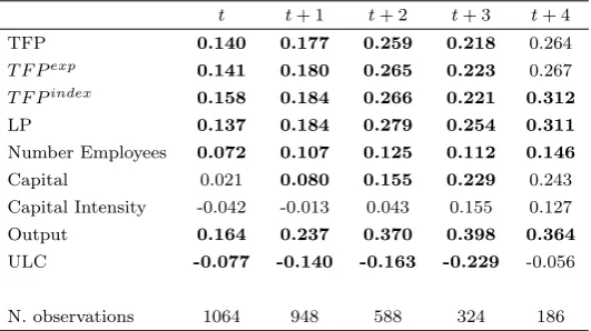
[image:19.595.166.432.364.513.2]

for matched controls because every starter is matched with one control unit, the single nearest neighbor. I consider four years after the starting year and I calculate ATT effects for the entry period (t), t+1 till the period t+4. PSM may fail considering a longer time horizon because of the restriction of the matched sample. Even if I am interested mainly on productivity indicators, I investigate also ATT effects for other firm characteristics, especially size and capital endowment.

Table 7: ATT Effects: PSM-DID estimates

t t+ 1 t+ 2 t+ 3 t+ 4 TFP 0.140 0.177 0.259 0.218 0.264

T F Pexp _0.141 _0.180 _0.265 _0.223 _0.267

T F Pindex _0.158 _0.184 _0.266 _0.221 _0.312

LP 0.137 0.184 0.279 0.254 0.311

Number Employees 0.072 0.107 0.125 0.112 0.146

Capital 0.021 0.080 0.155 0.229 0.243 Capital Intensity -0.042 -0.013 0.043 0.155 0.127 Output 0.164 0.237 0.370 0.398 0.364

ULC -0.077 -0.140 -0.163 -0.229 -0.056 N. observations 1064 948 588 324 186

Bold values are significant at least at 10%.

Bootstrapped standard errors are calculated (200 replications).

The results show that the average TFP effect of exporting is positive and statistically significant. Firms that start exporting grow more than firms that serve only the domestic market. There are also significant and positive effects on labour productivity, capital, size and output43_{. These positive}

effects are persistent and they last till the fourth year (third year for the capital and productivity) after the export entry44_{. Learning-by-exporting} 43_{The effects on TFP and labour productivity are very similar, this means that the}

export activity has no significant effect on the firm capital intensity, as it is directly shown in the table. DID results on the unmatched sample bear, as expected, a stronger impact on the firm efficiency. These results are available upon request.

44

(20)

hypothesis seems to be confirmed with every productivity indicator (LP, semiparametric TFP indicators and TFP index). When I match on the pooled sample, I obtain very similar ATT effects, only for the year t+3 the TFP effect become not significant. I have also tried to impose a tolerance level on the maximum propensity score distance (caliper) in order to face with the risk of bad matches if the closest neighbour is far away. I have used a caliper level of 0.01 and I have obtained the same results. This robustness checks confirms the goodness of my matching procedure45_.

The sample size decreases when I focus on periods more distant from the export entry (Table 7), this drop can be attributed to different reasons: starters can stop exporting after some years; the controls or starters can exit the market; or the time dimension of the database does not allow to follow the whole history of the firms after the export entry. In order to take into account these sources of sample selection, following De Loecker (2007), I have recalculated the post-entry effects for the different firms’ samples according to the number of years I can observe the starter after the export entry. Table 12 in the Appendix shows the relative results. The ATT effects are quite similar between the different samples, the only exception is for the sample of firms for which I can observe at least 5 consecutive export years after the export entry, even if this could be due to the small size of this sample.

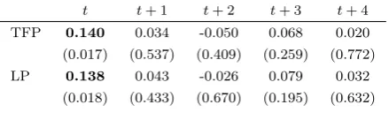
Looking at the previous results I could hypothesize that in the entry year firms place themselves on a higher TFP path and then they stay on this “superior” path (De Loecker, 2007). This idea seems to be verified when I calculate ATT effects on yearly TFP growth rates. Table 8 shows that starters present a significant higher annual growth rate than never exporters only for the entry period. Thus, in the entry year starters go on a higher TFP path and in the following period they stay on this path and confirm their advantage compared with never exporters.

4.1 Robustness tests

The ATT calculation is a superior and flexible approach, if compared with OLS regression, in estimating the conditional expectation of the outcome variable because it does not impose linear functional form restrictions. Any-way, as robustness check, I have also tried to implement a different

meth-reliable, probably due to the small sample size, because I have experimented some changes in magnitude and significance with different probit specification for export entry.

45_{When I restrict the matching imposing a caliper=0.01 the starters I can match drop}

(21)

[image:21.595.188.408.164.236.2]

Table 8: ATT effects: Yearly Growth Rates

t t+ 1 t+ 2 t+ 3 t+ 4 TFP 0.140 0.034 -0.050 0.068 0.020 (0.017) (0.537) (0.409) (0.259) (0.772) LP 0.138 0.043 -0.026 0.079 0.032

(0.018) (0.433) (0.670) (0.195) (0.632) Bold values are significant at least at 10%.

Bootstrapped standard errors are calculated (200 replications).

odology. Following studies of Greenaway et al. (2003, 2004) I have pooled my observations (of starters and matched controls) concerning different post-entry periods and I have estimated the regression:

∆T F Pit = α+

4

X

σ=0

βDt+σ +γDt−1_∗_{ST ART}

i+

4

X

σ=0

δDt+σ ∗ST ARTi+

+ϕT F Pi,t−1+θni,t−1+ιdr+µdj+ρdy +ǫijt (7)

where TFP growth is the dependent variable. Dt+σ are dummy variables assuming value 1 in the event time for never-exporters and exporters, these dummies capture the effect of events that occur in t+σ but are common to all firms46_. _{ST ART}

i is a time invariant dummy equal to 1 for starters and 0

for matched controls. The interaction Dt−1_∗_{ST ART}

i is 1 only for starters

in the period before export entry, this variable captures different pre-entry characteristics between starters and never exporters (if the matching was good it should not be significant). Dt+σ∗ST ARTi is equal to 1 in the

post-entry years for only exporters. I estimate this equation keeping in my dataset only starters and matched controls for the years −1 ≤ t ≤ 4: the pre-entry period, the entry year and the four years after entry 47_{. In this way, TFP}

growth of firms is compared with one of never-exporters in the pre-entry period (t-1). I control for the lagged level of TFP and lagged size, and I always include dummies for sector, region and year. I also try to take into account firm fixed effects. The coefficient of interest is δ showing the change in the TFP growth for starters in the post-entry period. Table 9 shows the productivity growth for starters and never exporters before and after entry.

46_{For example,}_D

t+3is equal to 1 in period t for starters if in t-3 they started exporting,

and it is equal to 1 also for exporters if in t-3 the related starters (which never-exporters is matched with) started exporting.

47

(22)

[image:22.595.199.390.164.224.2]

Table 9: Productivity Growth

N everExport. Starters

Before α α+γ

After α+β α+β+δ

With this regression I am analysing the annual growth rates. In opposite to Table 8, here I am considering together different post-entry years and I can also control for other additional regressors that could be affecting the firm performance over the period after export entrance (lagged TFP and size). Table 8 could be compared with the column 1 and 3 of Table 13 in the Appendix. This analysis further confirms the hypothesis on learning-by-exporting. I find a higher TFP growth rate for starters in the entry period, and when I control for lagged TFP and size I obtain significant export ef-fects also for the period t+1 and t+2. Adding firm-fixed efef-fects, significant post-entry effects are shown for the whole post-entry period.

4.2 A comparison between continuous exporters and

export stoppers

Thanks of the wide time dimension of the database I have estimated the post-entry effects for a 5-year interval after the export entry. In this interval some starters stop exporting. In the previous analysis I have calculated the productivity effects of starters till they stay in the export market, discarding the observations for starters after their exit from the export market, because my focus was on the potential gains for the firms while they are operating in the international context. Anyway, when I re-include these observations I still find positive post entry effects, even if they are a little downsized if com-pared with previous findings48_{. In this paragraph I also investigate if there}

exist some differences in post-entry effects between starters that continu-ously export and starters that stop exporting. I compare post-entry effects for these two starter groups and never exporters. I estimate the following

48_{These results are not shown, but are available upon request. The effects are the same}

(23)

regression:

∆T F Pit = α+

4

X

σ=0

βDt+σ +γDt−1

∗ST ARTi+δP OSTitCON T +ηP OSTitST OP +

where Dt+σ _and _{ST ART}

i are defined as in the equation 7; P OSTitCON T

and P OST_itST OP are dummies capturing the post-entry effects (with no dis-tinction according to the distance from export entry) respectively for starters which in my sample continuously export and starters which stop exporting after some years. I control for the lagged level of TFP and lagged size, and I always include dummies for sector, region and year. The analysis (Table 14 in the Appendix) confirms that there are no differences in the average yearly post-entry effects between the two types of starters. I have already verified that the jump in the productivity concerns the export entry year, then exporters stay on this superior productivity path without any great difference in the following growth rates (if compared with never exporters). In the last two columns of table 14 in the Appendix I show results of the following regression:

∆T F Pit = α+

4

X

σ=0

βDt+σ +γDt−1_∗_{ST ART}

i+δP OSTitST AY +ηP OSTitEXIT +

In this case I split the post-entry effects for starters while they are still ex-porting from the effects following their export exit (for starters that stop exporting after some years). Especially P OST_itST AY is a dummy equal to 1 for all starters (both continuous exporters and stoppers) till they are in the export market, while P OST_itEXIT captures the productivity effects for starters after they stop exporting. Results confirm that there are positive ef-fects while starters are in the export market, but after they stop exporting no significant difference is found between stoppers and never exporters. Anyway also the significant higher productivity growth for starters while they are in the export market is likely to be driven by the effects of the first (and second) post-entry year.

5 In search of learning channels

5.1 The link between exports and imports

(24)

entry year. In this section, I want both to test if post-entry effects, I found previously, are driven by export entry and not import entry and I try also to verify if firms which start importing in combination with exporting obtain larger gains.

In previous sections, I have checked for the lagged import status. Includ-ing in the probit specification the lagged import dummy, I have taken into account previous import activity of matched and control units. As Table 6 has shown, there is no a significant difference in the import status between starters and never exporters after matching, so post-entry effects are cleaned for the previous firm import status49_{. Anyway, even if the matching}

pro-cedure let me to control for pre-entry characteristics, it does not check for events that could happen in combination with export entry, in particular for current import entry. In this section, I want to test if the current import status (in t) could affect, in combination with exporting, post-entry effects, and could contribute to explain them. I split starters’ sample in two groups: the first group include export starters which start also importing in t (they did not import in t-1, but import in t); the second firm group includes the other firms (firms that already imported in t-1 and continue importing, and firms that import neither in t-1 nor in t50_{). In both groups I have obviously}

included the relative matched controls51_{. My previous results are generally}

confirmed (Table 10) also when I drop, from my sample, firms which start importing and exporting at the same time, even if now post-entry effects are slightly downsized and there is no significant effect in t (Group2)52_{. This}

finding further supports the existence of significant positive effects stemming from export activity, and I can reject the hypothesis that efficiency improve-ments previously found are only driven by firms’ foreign sourcing. Anyway, I also verify larger productivity gains for firms which start exporting and importing at the same time. This analysis represents a robustness check of previous results, but also shed some light on the nexus between exports and imports: participation in export market increase the firm performance, and these improvements of productivity could be higher if firms turn to more complex internationalisation strategies.

49_{Even if I have not matched exactly on the lagged import status, I can see from Table}

6 that the matching on this variable was quite perfect.

50

The previous import status does not represent a problem for the interpretation of the post-entry effect I previously found because I have already controlled for the previous import activity in t-1 in the matching procedure.

51_{The matching procedure is not changed.}

52_{I calculate ATT effects until t+2, because the two samples are too small for following}

(25)

[image:25.595.220.374.165.242.2]

Table 10: ATT effects: Control for the current import status

TFP

t t+ 1 t+ 2 Group1 0.206 0.239 0.210

(0.010) (0.016) (0.093) Group2 0.109 0.156 0.229

(0.172) (0.084) (0.042)

Group1 = New Importers. Group2 = Old Importers and Non Importers. Bootstrapped standard errors are calculated. Bold values are significant at least at 10%.

5.2 Learning-by-exporting: the role of the

technolo-gical gap

In this section I focus on recent studies trying to highlight the importance of domestic and foreign context in explaining the potential export effects. On one hand, Greenaway and Kneller (2007) have investigated if industry differences can explain the existence of efficiency improvements after export market entry: they find that productivity gains for exporters are lower in industries already exposed to high levels of trade and to high levels of R&D

(26)

trade partners are European countries and, in general, advanced countries53_.

I can suppose that, in sectors where Turkey has no a comparative advantage, Turkish firms are less productive, in average, than foreign firms; in opposite in comparative advantage sectors Turkish productive system is more efficient (in absolute or relative terms) than foreign productive systems54_.

I want to verify if learning effects are larger and significant for new ex-porters in comparative disadvantage industries because in these sectors the productivity gap between the domestic productive system and foreign pro-ductive systems should be higher than in comparative advantage sectors. New exporters, in comparative disadvantage industries, could be exposed to a more competitive environment than their domestic context and could be more exposed to positive spillovers, this could explain larger post-entry effects stemming from exporting. As a consequence, I could expect learning-by-exporting to be more intensive in comparative disadvantage sectors. I have split sectors according to the comparative advantage. In order to take into account the Turkey’s pattern of comparative advantage (and disadvant-age) across industries, I have used the trade flows and I have calculated the “index of revealed comparative advantage” (henceforth RCA)55_. Com-53_{Turkish exports to OECD countries in manufacturing sector represent 80% of total}

exports.

54_{This means that in comparative advantage sectors Turkish firms could be more}

pro-ductive in average than firms of trade partner countries or, even if they could be less efficient than foreign firms, the differential of productivity should be lower than in com-parative disadvantage sectors. Mayer and Ottaviano (2007) report that “The concepts of comparative advantage and comparative disadvantage are used to identify industries in which a country is stronger than its competitors and those in which it is weaker, meaning industries in which its relative costs of production are respectively low and high”. They compare RCA (revealed comparative advantage), built on trade data, with ECA (estim-ated comparative advantage), built on productivity data, for Italy and UK and show a positive correlation.

55

The RCA is defined as

RCAi=

XT U R,i/XT U R

XW,i/XW

(10)

where XT U R,i andXW,iare the exports of Turkey and of the comparison group of

coun-tries in the industryi, whileXT U RandXW are the exports of Turkey and the comparison

(27)

parative advantage index can give an idea about the comparison between domestic market and foreign markets in every sector, and it can show the technological gap of Turkish industries to frontier. I assume firms are more distant to frontier in comparative disadvantage sectors. After the matching procedure shown in section 4, I define postCA a vector of dummy variables for the post-entry period for starters in comparative advantage (CA) sectors, and postCD a similar vector for the post-entry period for starters in compar-ative disadvantage sectors (CD). I can calculate post-entry effects with the following equation:

∆T F Pi,s=α+β1postCAi,s+β2postCDi,s+ǫis (11)

where ∆T F Pi,s is the productivity growth between every post-entry year

and pre-entry (t-1) year56_{. The variable TFP is always expressed as a}

devi-ation from the industry-year mean, in order to capture and correct for effects that are common to all firms belonging to the same sector (especially, in order to correct for specific effects linked to comparative advantage sectors or comparative disadvantage sectors). I am analysing the change in pro-ductivity following export entry compared with pre-entry period. I consider separately post-entry effects between starters in comparative advantage sec-tors and starters in comparative disadvantage secsec-tors for every year after export-entry (till the fourth year after the entry). The coefficient β1

cap-tures the average change in performance indicators related to the entrance in the export market for starters in comparative advantage sectors, while the coefficientβ2 can be interpreted as the same effect for starters in comparative

disadvantage sectors. Estimated coefficients on dummy variables postCAi,s

andpostCDi,shave to be interpreted as efficiency differentials with respect to

the omitted group, that is never exporters. We run simple OLS regressions57_.

For the entry year starters in CA sectors are improving their productiv-ity if compared with non-exporters, while there are no significant effects for starters in CD sectors (Table 11). In following years, effects in CA indus-tries turn to be non significant, while in CD sectors exporters start having significant effects since t+1 and it seems they continuously increase their

except footwear (ISIC 322); Rubber products (ISIC 355); Manufacture of Non-Metallic Mineral product, except product of petroleum and coal (ISIC 361; ISIC 362; ISIC 369). The pattern of comparative advantage is quite constant during the sample period.

56_{For the entry period it is calculated as ∆}_{T F P}

i,0 =tf pi,t−tf pi,t−1, where tfp is in

logarithms. For the first year following the entry it is calculated as ∆T F Pi,1 =tf pi,t−

tf pi,t−2and so on. 57

(28)

[image:28.595.120.471.165.260.2]

Table 11: ATT Effects: Comparative Advantage

t t+ 1 t+ 2 t+ 3 t+ 4 TFP Starters CA 0.180 0.187 0.264 0.059 0.086 Starter CD 0.104 0.157 0.254 0.352 0.399

CumTFP Starters CA 0.180 0.307 0.476 0.378 0.715 Starter CD 0.104 0.341 0.609 0.818 1.467

Bold values are significant at least at 10%.

efficiency. The analysis shows that firms in CA sectors can take advantage from the export activity immediately when they enter foreign markets, in opposite it seems that firms in CD sectors need some time in order to ex-ploit the opportunities offered by foreign markets. Thus, I verify a different timing of post-entry effects for different sectors. In CD sectors firms are not able to absorb immediately spillovers from international markets (new tech-nologies, new production strategies), because the gap with foreign markets in these sectors could be large and they have to accomplish some efforts in order to prepare themselves to take advantage from the new context. In opposite, in CA sectors firms does not face any difficulty in exploiting the potential of learning. Anyway when starters in CD industries are ready to absorb spillovers from the new context they can exploit a higher potential of learning than firms in CA industries. This hypothesis seems to be con-firmed when I analyse the cumulative productivity58_{of firms (always splitting}

between starters in CA and CD sectors).

6 Concluding remarks

The paper analyses the link between exports and firm performance for a middle income country, Turkey. Both self-selection and post-entry effects are important drivers behind the positive correlation found between export involvement and firm productivity. The work contributes especially to

sup-58_{The cumulative productivity is calculated as}

CumT F Pi,s = s

X

δ=0

tf pi,t+δ−tf pi,t−1

(29)

port the hypothesis of a potential for learning stemming from export activity when the analysed country is not at the technological frontier and confirms results highlighted by previous papers. Export starters show a higher per-formance in the post-entry period. It seems export activity places firms on a superior productivity path in the entry year and then they stay on this path in the following period.

My analysis displays also a strict linkage between export and import entry. Firms often start importing and exporting at the same time and it is important to control for this simultaneity in the analysis of post-entry effects. A deeper investigation confirms that productivity gains also hold when I take into account the current import status. In addition the benefits seem to be larger when firms are involved in both international strategies. The relationship between export and import activity at the firm level has received scarce attention, but it could become an important research field in the future.

Finally, I try to shed some light on the channels of learning-by-exporting and I look for an heterogeneity in post-entry effects according to the sectoral differential of performance between the domestic context and foreign markets. I verify a different timing of productivity improvements across sectors: new exporters in comparative disadvantage sectors take more time to reap the benefits of export entry, but, in the “long” term, the potential of learning could be larger than in comparative advantage industries because the distance to frontier is higher. This finding supports the hypothesis that competition and technology spillovers are significant channels through which exports may affect firm’s productivity.

References

[1] Aldan, A. and M. Gunay, 2008. Entry to Export Markets and Pro-ductivity: Analysis of Matched Firms in Turkey. The Central Bank of the Republic of Turkey, Working Paper 08/05.

[2] Alvarez, R. and R. Lopez, 2005. Exporting and Performance: Evid-ence from Chilean Plants. Canadian Journal of Economics 38(4), 1384– 1400.

(30)

Discussion Paper 5065.

[4] Aw, B.Y., S. Chung, and M. Roberts, 2000. Productivity and Turnover in the Export Market: Micro Evidence from Taiwan and South

Korea. The World Bank Economic Review 14(1), 65-90.

[5] Becker, S.O. and A. Ichino, 2002. Estimation of average treatment effects based on propensity scores. The Stata Journal 2(4), 358-377. [6] Bernard, A. and B. Jensen, 1999.Exceptional exporters performance:

cause, effect or both?. Journal of International Economics 47(1), 1-25. [7] Bernard, A., J. Eaton, B. Jensen, and S. Kortum, 2003. Plants

and Productivity in International Trade. American Economic Review 93(4), 1268-1290.

[8] Blalock, A. and J.B. Jertler, 2004.Learning from exporting revis-ited in a less developed setting. Journal of Development Economics 75(2), 397-416.

[9] Blundell, R. and M. Dias, 2000. Evaluation methods for non-experimental data. Fiscal Studies 21(4), 427–468.

[10] Caliendo, M. and S. Kopeinig, 2008. Some practical guidance for the implementation of propensity score matching. Journal of Economic Surveys 22(1), 31-72.

[11] Castellani D., 2002. Export behavior and productivity growth: Evid-ence from Italian manufacturing firms. Review of World Economics 138(4), 605–628.

[12] Castellani D., Serti F. and C. Tomasi, 2008. Firms in Interna-tional Trade: Importers and Exporters Heterogeneity in the Italian

(31)

[13] Clerides, S., S. Lach, and J. Tybout, 1998. Is learning by ex-porting important? Microdynamic evidence from Colombia Mexico and

Morocco. Quarterly Journal of Economics 113(3), 903-948.

[14] Damijan, J.P. and C. Kostevc, 2005. Performance on Exports: Continuous Productivity Improvements or Capacity Utilization. LICOS Discussion Paper 16305.

[15] Delgado, M., J. Farinas, and S. Ruano, 2002. Firm productivity and export markets: a non-parametric approach. Journal of International Economics 57(2), 397-422.

[16] De Loecker, J., 2007. Do Exports Generate Higher Productivity? Evidence from Slovenia. Journal of International Economics 73(1), 69-98.

[17] Fernandes, A. and A. Isgut, 2007. Learning-by-Exporting Effects: Are They for Real?. MPRA Paper 3121.

[18] Girma, S., D. Greenaway, and R. Kneller, 2003. Export market exit and performance dynamics: a causality analysis of matched firms. Economics Letters 80(2), 181-187.

[19] Greenaway, D. and R. Kneller, 2007. Industry Differences in the Effect of Export Market Entry: Learning by Exporting? Review of World Economics 143(3), 416-432.

[20] Greenaway, D. and R. Kneller, 2008.Exporting, productivity and agglomeration. European Economic Review 52(5), 919-939.

[21] Good, D.H., M. Nadiri,and R. Sickles, 1997. Handbook of Applied Econometrics: Micro-econometrics. Blackwell: Oxford.

(32)

[23] Kasahara H. and J. Rodrigue, 2008. Does the use of imported intermediates increase productivity? Plant-level evidence. Journal of De-velopment Economics 87, 106-118.

[24] Kraay, A., 1999. Exportations et Performances Economiques: Etude dun Panel dEntreprises Chinoises. Revue d’Economie du Developpement 1–2, 183-207.

[25] Levinsohn, J. and A. Petrin, 2003. Estimating Production Func-tions Using Inputs to Control for Unobservables. Review of Economics Studies 70(2), 317–341.

[26] Mayer, T. and G.I.P. Ottaviano, 2007. The Happy Few: The in-ternationalisation of European firms. Bruegel Blueprint Series.

[27] Melitz, M., 2003.The Impact of Trade on Intra-Industry Reallocations and Aggregate Industry Productivity. Econometrica 71(6), 1695–1725. [28] Muuls, M. and M. Pisu, 2009. Imports and Exports at the Level of

the Firm: Evidence from Belgium. World Economy 32(5), 692–734. [29] Pavcnik, N., 2002. Trade Liberalization, Exit, and Productivity

Im-provements: Evidence from Chilean Plants. Review of Economic Studies 69(1), 245-276.

[30] Rosenbaum, P. and D. Rubin, 1983. The central role of the propensity score in observational studies for causal effects. Biometrica 70(1), 41-55.

[31] Serti, F. and C. Tomasi, 2008. Self Selection and Post-Entry effects of Exports. Evidence from Italian Manufacturing firms. Review of World Economics 144(4), 660–694.

(33)

[33] Taymaz, E. and K. Yilmaz, 2007.Productivity and trade orientation: Turkish manufacturing industry before and after the customs union. The Journal of International Trade and Diplomacy 1(1), 127–154.

[34] Van Biesebroeck, J., 2005. Exporting Raises Productivity in sub-Saharan African Manufacturing Firms. Journal of International Econom-ics 67(2), 373–391.

[35] Wagner, J., 2002. The causal effects of exports on firm size and labor productivity: first evidence from a matching approach. Economics Letters 77(2), 287-292.

[36] Wagner, J., 2007a.Exports and productivity: A survey of the evidence from firm level data. World Economy 30(1), 60–82.

[37] Wagner, J., 2007b. Exports and Productivity in Germany. Applied Economics Quarterly 53(4), 353–373.

(34)