Improved Clustering Algorithm Based on Density Isoline

http://dx.doi.org/10.4236/ojs.2015.54032

Improved Clustering Algorithm Based on

Density-Isoline

Bin Yan, Guangming Deng

College of Science, Guilin University of Technology, Guilin, China Email: [email protected]

Received 8 April 2015; accepted 7 June 2015; published 10 June 2015

Copyright © 2015 by authors and Scientific Research Publishing Inc.

This work is licensed under the Creative Commons Attribution International License (CC BY). http://creativecommons.org/licenses/by/4.0/

Abstract

An improved clustering algorithm was presented based on density-isoline clustering algorithm. The new algorithm can do a better job than density-isoline clustering when dealing with noise, not having to literately calculate the cluster centers for the samples batching into clusters instead of one by one. After repeated experiments, the results demonstrate that the improved density-isoline clustering algorithm is significantly more efficiency in clustering with noises and overcomes the drawbacks that traditional algorithm DILC deals with noise and that the efficiency of running time is improved greatly.

Keywords

Density-Isolines, Density-Based Clustering, Clustering Algorithm, Noise

1. Introduction

Clustering is a modern multivariate statistical method in studying the similarity of different samples, which groups a set of objects into classes or clusters such that objects within a cluter have high similarity in compari-son to one another, but they are dissimilar to objects in other clusters. Clustering is widely used in pattern rec-ognition, data mining, machine learning and image segmentation. According to this thought clustering algorithm is generally classified into partition, hierarch, density-based, grid-based and model-based clustering [1]. Parti-tion methods such as K-means [2] find shaped clusters only. Hierarchical clustering methods [3] discovered clusters by merging the closet pair of clusters iteratively until the desired number of clusters was obtained. Grid- based clustering such as STING requires the data must be intensive in space.

drawback, OPTICS was proposed in [5]. While expanding a cluster, OPTICS selects each point to be expanded in increasing order of its distance to the current cluster and changes ε for identifying ε-neighborhood gradually. If ε grows rapidly, it stops expanding the cluster and starts another one. However, OPTICS can not be paralle-lized using Map Reduce easily since it always has to merge point one by one serially to the current cluster to determine where to separate the cluster. Both DBSCAN and OPTICS discover the clusters which are dense re-gions of data points and separated by sparse rere-gions with respect to given density parameters [1].

Jain had proposed a density-based clustering algorithm which divided samples into sever regions then merger into different clusters. The size of the region in this algorithm plays an important role, and the clusters are mea-ningless when the sizes of regions are too big and complexity of the algorithm will increase while the sizes are too small. Besides, [6] proposed a density-based clustering algorithm which merges points by “density-reach- able” and “density-connected”, however, it can not deal with samples with high dimensions. Density-based clu- stering can easily find out clusters of different shapes and sizes, however, most of them can not handle the data-base with varying densities and high dimensions.

Clustering algorithm based on density-isoline (DILCA) [7] was a new density-base algorithm proposed by Yanchang Zhao. The core thought of this algorithm is: calculate out the density value of each sample according to the distance of every two samples and given neighborhood radius; then search out the points whose density values are bigger than density threshold; next, merge the points which are overlap according to the neighbor-hood radius R; finally we can get the initial clusters. Those samples that don’t belong to any clusters are called noises. When compared with DBSCAN and OPTICS, DILCA needn’t input any parameters and is an unsuper-vised algorithm. Although this algorithm can handle the databases with high dimensions and varying densities, it fails to deal with the noises. In other words, not all samples are merged into clusters.

Being inspired by the recent trend of research in the clustering, in this paper we suggested an improved clus-tering algorithm based on density-isoline (IDILCA) which can successful deal with noises as well as accelerate the merge process by batching into clusters instead of one by one. The main steps of IDILCA are as follows:

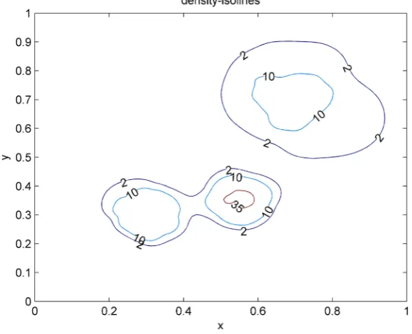
[image:2.595.164.464.461.704.2]

Step 1. The samples within density-isoline threshold are batched into clusters. The number of clusters is con-firmed by threshold with minimum density-isoline value which is in demand. All the samples whose density values are bigger than the density-isoline threshold are merged once and for all. In Figure 1, if we set densi-ty-isoline threshold as 10, the samples can divided into three independent parts A, B and C. Therefore, we can merge all the samples within the part A into the same category once and for all. In a same way we can get the in-itial category B and C.

Step 2. The noises merge into clusters one by one. Those samples whose density values are below the thre-shold are called noises. When merging the noises into category we use “the minimum density-reachable-dis- tance” principle; that is to say, calculating out the density-reachable-distance of every noise and each initial cat-egory, then merging the point into the nearest one, until all the samples have merged into categories.

2. Related Work

Clustering algorithm based on density-isoline (DILCA) was proposed in [7] by Yanchang Zhao. Being a new clustering algorithm, DILCA starts from the density-isoline map of samples and find relatively dense regions which are clusters. DILCA is capable of eliminating outlines and discovering clusters of various shapes as well as varying density distribution. It is an unsupervised clustering algorithm because it requires no input parameter. The DILCA algorithm is described as follows:

Step 1. Calculating out the distance of every two samples, and then we can get a distance matrixDist. (The distance is described by Euclidean distance)

Step 2. Confirming the size of neighborhood radius Rt according to the distance matrix. Step 3. Calculating the density value matrixDen.

Step 4. Confirming the density threshold DT according to density value matrix.

Step 5. Merging: if the density value of sample A and sample B is bigger than threshold DT respectively, and the distance between A and B is smaller than Rt, then merge A and B to a same category.

Step 6. If the result we get is not satisfied, we can adjust the density threshold, until get the result that we wanted.

The DILCA has been successfully to find out the clusters with varying density, shape and size. However, it fails to deal with noise that is to say not all samples take the merging progress. Besides, the computational com-plexity associated with this algorithm is high, it required a long compute time when the database is very big. Thus the algorithm needs improvement.

3.

IDILCA

: An Improved Clustering Algorithm Based on Density-Isoline

3.1. Definitions

Let D=

{

p p₁, ₂,,pn

}

be a collection of d-dimensional points. Each point pi∈D is represented as a vector

( ) ( )

1 , 2 , ,

( )

3

i i i

p p  p where P j_i

( )

represents the j-th coordinate of the point.

Definition 3.1. The distance between sample P_i and sample P_j is defined as

(

)

(

( )

( )

)

2

(

( )

( )

)

2

(

( )

( )

)

2

, 1 1 2 2

i j i j i j i j

d p p = p −p + p −p + + p d −p d

Definition 3.2. The neighborhood threshold is defined as

( )

mean

coefR d R

n

=

where mean

( )

d represents the mean value of the whole distances between every two samples.𝑛𝑛represent the number of samples. coef R∈

( )

0,1 represents the adjust coefficient of neighborhood radius, according to [7], when coef R=0.3 we can get a satisfied result in most conditions.

Definition 3.3. The density of a sample is calculated by the density distribution of the neighborhood, that is to say the distance to the sample from the neighborhood, which is less than the points of a fixed value, serves as neighborhood distribution density of the sample.

( )

i

(

{

j

(

i, j

)

}

)

Dens p =Num p d p p <Rt

where we will represent P_i and P_j as input samples, Dens p

( )

_i represents the sample’s density distribution in P_i’s neighborhood. Rt represents the distance threshold.

Definition 3.4. Density directly-reachable

Definition 3.5. Density-reachable

A point p is density-reachable from a point q if there is a sequence of data point

(

z z₁, ₂,,zj

)

with z1=p and z_j=q such that z_j+1 is directly density-reachable from z_j.

Definition 3.6. Density-reachable distance

If p is density-reachable from q, then the density-reachable distance between p and q is defined as

(

,

)

1

(

, 1

)

n

i i i

d p q =

∑

= zd p p+

where zd p q

(

,

)

was defined in Definition 3.4 and pi is a sequence of data point p p1, 2,,pj with p1= p and p_j =q.

3.2. Confirm the Number of Clusters

How to determine the number of clusters as well as choose the initial cluster centers are very important for the final clustering results. IDILCA is a new algorithm starts from density-based algorithm and combined with con-tour. When depicting the mountains and the oceans, we usually use contours. As we all know, every point has the same altitude from a contour. Similarly, if the samples have the same density value, we connecting them with a line, which we call isoline. The concrete progress is described as follow:

Step 1. Calculating the density values for each sample.

Step 2. Connecting the points with a line if they have the same density values, thereby we get the isolines. Step 3. Choosing a suitable isoline as the threshold, the criterion of suitable is decided by isolines, if the iso-line divides the samples into k independent portions then the number of cluster is k and the area within isoiso-line we regard them as initial cluster centers.

This method can efficiently help us confirm the number of clusters as well as calculate the initial cluster cen-ters. As we can see in Figure 1, when we choose 20 as threshold, the samples divided into 3 categories, if we choose 10 as the threshold, the number of clusters is 2.

3.3.

IDILCA

Algorithm

Based on DILCA algorithm and some further improvement were made, the IDILCA has a faster operation speed as well as stronger ability when dealing with noises. The basic thought of IDILCA algorithm is: calculating the density values of each sample and connecting the points with isolines if they have the same density values, then merge the points into clusters according to the isoline-threshold, thereby we get the initial clusters. As for those points that do not belong to any clusters are called noises. Before merging the noises, we calculate their density reachable distance to the initial clusters and then merging it into the cluster one by one according to the “mini-mum density-reachable distance” principle. The concrete progress is described as follow:

Step 1. Calculating the distance of every two samples and then we get the distance matrixDist. Where

(

i, i

)

(

i, j

)

Dist p p =d X X ;

Step 2. Confirming the neighborhood radius length according to the distance matrix from step 1.

(

)

(

coefR

)

R=mean Dist n ;

Step 3. Calculating the density values of each sample and then getting the density value matrixDen. Where

( )

i

(

{

j|

(

i, j

)

}

)

Dens p =Num p d p p <R ;

Step 4. Drawing the density-isoline according to the density value matrix from step 3; Step 5. Confirming the number of clusters k according to density-isoline;

Step 6. Selecting the minimum density-isoline value that separates the samples into k independent area as the isolines threshold value;

Step 7. Merging all the samples that within the density-isoline threshold into a same category once and for all and calculating the initial cluster centuries;

Step 8. Recalculating the density-reachable distance between the rest samples with the initial clusters, and then we can get the density-reachable distance matrixDist. Where Dist p G

(

i, j

)

=rd p G

(

j, j

)

;

Step 9. Merging the noise into the category one by one according to minimum density-reachable distance principle;

3.4. Related Formula

Let m be the density-isoline threshold and the samples separate into k independent area, then we confirm the number of clusters is k. Let the i-th

(

i=

(

1, 2,,d

)

)

independent area conclude n_i samples, then we can get the j-th coordinate of category G_i as follow

( )

1

(

( )

)

i i

i i

x G i

G j P j

n ∈

=

_∑

where P j_i

( )

represent the j-th coordinate of sample P_i. The initial cluster century of G_i is described by

( ) ( )

( )

(

G_i 1 ,G_i 2 ,,G d_i

)

For the noise, we defined the density-reachable distance between j-th sample and category G_i as

(

,

)

(

,

)

(

, 1

)

i i

i i i

p G q G

d p G rd p q zd z z₊ ∉

∈

= =

∑

where zd p q

(

,

)

was defined in Definition 3.4 and z_i is a sequence of data point z z₁, ₂,,z_j with z₁=p and z_j=q.

As for the number of category is clear and we can also calculate the initial cluster century, so which category should the noise sample belong to is defined as

(

)

(

)

(

)

min d p G_j, _i →p_j∈G i_i =1, 2,,k

The final cluster is defined as

( )

(

)

1 i i ij i p G i

G p j

n ∈

=

_∑

4. Performance Analyses

The run time of the new algorithm mainly depends on calculating the matrix of the distance between any two samples. If the sample size is n, the final distance matrix is a matrix of n n× , and its time complexity is

( )

2

O n . When the sample size is very large, we can regard the distance matrix as an integer in order to save storage space, so the distance between two samples is only two bytes, which can greatly save memory space. In addition, because the clustering method is a batch clustering within the density threshold, the proportion of the noise sam-ples is small (typically within 10%), therefore, for the samsam-ples are batched into clusters,it can reduce the itera-tive process and save the iteraitera-tive time.

5. Experimental Results

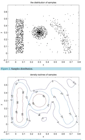
The experiment conduct on MATLAB 7.10.0 and the PC is HP Z600. The experimental data are synthesized which are based on certain shapes. There are 1360 sample points totally in Figure 2. Among them, 600 points show columnar distribution on the left side; 500 points present globular distribution in the middle; 200 points present arc distribution on the right side, and the rest 60 samples are noises of the random sample.

Experimental methods: 1) Comparing the result of the final clustering between the new algorithm and the original algorithm; 2) Comparing the consumed time between the new algorithm and the original one under the same sample size and environment.

[image:6.595.170.470.80.570.2]

Figure 2. Samples distribution.

Figure 3. Density-isolines of samples.

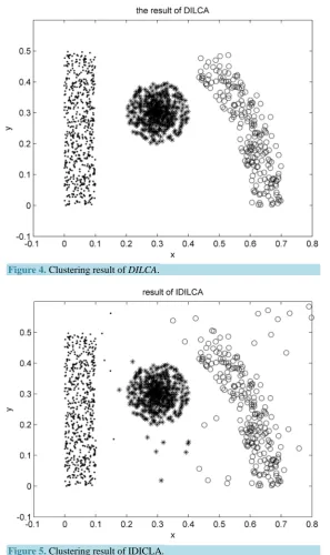
recalculate the density-reachable distance of the remaining samples (noise) and mergeit into the clusters accord-ing to the nearest “density-reachable distance” principle. The clusteraccord-ing result of the DILCA is shown inFigure 4 and the clustering result of the IDILCA by using the same data is shown inFigure 5.

By comparing the clustering results of the Figure 4 with the Figure 5, IDILCA not only have a well cluster-ing effect and can increase the function which deal with the noise but also can make all the samples join in the process of clustering.

[image:7.595.167.465.80.581.2]

Figure 4. Clustering result of DILCA.

Figure 5. Clustering result of IDICLA.

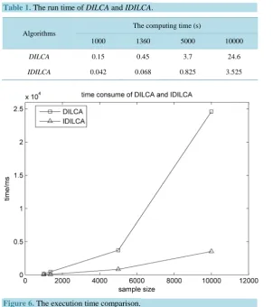
From Table 1, we can see the time complexity of IDILCA is less than the DILCA. This advantage is more prominent along with the increase of the sample size in Figure 6.

With the increase of the sample size, the original DILCA requires to iterate repeatedly in the process of the sample merging into the cluster. However, most samples batch into the clustersonce and for all in the improved IDILCA algorithm, which can save the iteration time by a computer.

6. Conclusion

[image:8.595.168.471.82.423.2]

Table 1.The run time of DILCA and IDILCA.

Algorithms

The computing time (s)

1000 1360 5000 10000

DILCA 0.15 0.45 3.7 24.6

IDILCA 0.042 0.068 0.825 3.525

Figure 6. The execution time comparison.

on density-isoline. It doesn’t require any input parameters and supports the users in determining appropriate values for it. After repeated experiments, the results of our experiments demonstrate that IDILCA is significantly more efficiency in clustering with noises. The new algorithm can not only make all the samples participate into clusters but also will not be affected by the shape of sample distribution and density distribution. The experi-mental results show that the new algorithm overcomes the drawbacks that traditional algorithm DILCA deals with the noise and the efficiency of run time is improved greatly.

References

[1] Han, J. and Kamber, M. (2006) Data Mining Concepts and Techniques. 2nd Edition, Margan Kaufmann Publishers, San Francisco.

[2] Macqueen, J. (1967) Some Methods for Classification and Analysis of Multivariate Observations. Fifth Berkeley Sym-posium on Mathematic Statistics and Probability, University of California Press, Berkeley, 666.

[3] Guha, S., Rastogi, R. and Shim. K, (2001) Cure: An Efficient Algorithm for Large Databses. Information Systems, 26, 35-58.http://dx.doi.org/10.1016/S0306-4379(01)00008-4

[4] Ester, M., Kriegel, H.P., Sander, J. and Xu, X. (1996) A Density Based Algorithm for Discover Clusters in Large Spa-tial Datasets with Noise. Proceedings of International Conference on Knowledge Discovery and Data Mining, 226- 231.

[5] Ankerst, M., Breunig, M.M., Kriegel, H.-P. and Sand, J. (1999) OPTICS: Ordering Points to Identify the Clustering Structure. SIGMOD Conference, 28, 49-60.http://dx.doi.org/10.1145/304182.304187

[6] Nanda, S.J. and Panda, G. (2014) Desugn of Computationally Efficient Density-Based Clustering Algorithms. Data & Knowledge Engineering, 1-16.