Probabilistic Analysis of a Computer System with Inspection and Priority for Repair Activities of H/W over Replacement of S/W

(1)

Probabilistic Analysis of a Computer System with

Inspection and Priority for Repair Activities of H/W over

Replacement of S/W

Jyoti Anand

Department of Statistics M.D.University,Rohtak-124001

Haryana (India)

S.C.Malik

Department of Statistics M.D.University,Rohtak-124001

Haryana (India)

ABSTRACT

The main aim of this paper is to carry out the probabilistic analysis of a computer system of two identical units in which one is operative and the other is in cold standby. In each unit h/w and s/w components fail independently and work together. A server visits the system immediately to inspect the h/w components at their failure to see the feasibility of repair. If repair of the h/w is not feasible, it is replaced by new one in the unit. However, only replacement of the s/w components is made by new one at their failure. Priority to the replacement and repair of the h/w components is given over the replacement of the s/w components. All the failure time distributions are assumed to be negative exponential while that of inspection, repair and replacement times are taken as arbitrary. Some reliability and economic measures of system effectiveness are evaluated using semi-Markov process and regenerative point technique. The graphs are drawn for a particular case to show the behavior of MTSF, availability and profit of the system models.

General Terms

Reliability and Economic Measures

Keywords

Computer System, Hardware and Software Failures, Feasibility of Repair, Priority for Replacement, Repair and Inspection, Probabilistic Analysis.

1. INTRODUCTION

In spite of increasing development and availability of new computer technologies, a little work has been dedicated to the probabilistic analysis of a computer system with independent failure of h/w and s/w components. And, most of the research work in the subject of h/w and s/w reliability has been limited to consideration of either h/w subsystem alone or s/w subsystem alone. Friedman and Tran[1] and Wilke et al. [2] tried to establish a combined reliability model for the whole system introducing both h/w and s/w under the assumption that h/w and s/w subsystems are independent to each other. Recently, Malik and Anand et al.[3,4] have suggested some reliability models of a computer system with independent h/w and s/w failures. In these models replacement of the components by new one is made in negligible time if inspection reveals that repair of h/w components is not feasible. However, in paper [4], priority for the replacement at s/w component is also made by new one over repair and replacement activities of h/w failures. But the concept of priority to repair activities of the h/w over replacement of the s/w has not been studied so far by any researcher in the subject of reliability.

In view of above, the present paper deals with the probabilistic analysis of a computer system considering the concepts of priority for the replacement and repair of the h/w components subject to inspection over replacement of the s/w. For this, a probabilistic model is developed by taking two identical units of a computer system. Initially, one unit is operative and other is kept as cold standby. Each unit has direct independent complete failure from the normal mode. There is a single server who visits the system immediately to do inspection. If repair of the defective h/w components is not feasible, it is replaced by new one. However, only replacement of the s/w components is made by new one whenever they fail. The priority is given to replacement and repair of the h/w components subject to inspection over replacement of the s/w components at their failure. The failure, repair and inspection time are taken as independent and uncorrelated random variables. The failure time of the unit follow negative exponential distributions while that of repair, inspection and replacement s/w and h/w are taken as arbitrary. To analyze the system probabilistically in detail, expression for some reliability characteristics such as mean sojourn times, mean time to system failure (MTSF), availability, busy period of the server due to h/w failure or due to s/w failure, expected no. of replacement due to h/w failure or due to s/w failures & expected no. of visits by the server are derived by making use of semi-Markov process and regenerative point technique. The graphs are drawn for a particular case to show the behavior of MTSF, availability and profit of the system models.

2. NOTATIONS

E : The set of regenerative states

O : The unit is operative and in normal mode

cs : The unit is cold standby

a/b : Probability that the system has hardware /

software failure

1/2 : Constant hardware / software failure rate

p/q : Probability that repair of the unit due to

hardware failure is not feasible / feasible

FHUr/FHUR : The unit is failed due to hardware and is

under repair /under repair continuously from

(2)

FHUi/FHUI : The unit is failed due to hardware and is

under inspection/ under inspection

continuously from previous state

FHWi/FHWI : The unit is failed due to hardware and is

waiting for inspection/ waiting for

inspection continuously from previous

state

FSURp/FSURP : The unit is failed due to the software and

is under replacement/under replacement

continuously from previous state

FHWRp/FHWRP : The unit is failed due to the hardware and

is waiting for replacement/waiting for

replacement continuously from previous

state

h(t) / H(t) : pdf / cdf of inspection time of unit due to

hardware failure

f(t) / F(t) : pdf / pdf of replacement time of the

software

g(t) / G(t) : pdf / cdf of repair time of the unit due to

hardware failure

qij / Qij(t) : pdf / cdf of passage time from

regenerative state i to a regenerative

state j or to a failed state j without

visiting any other regenerative state in

(0, t]

qij.kr/Qij.kr : pdf/cdf of direct transition time from

regenerative state i to a regenerative state

j or to a failed state j visiting state k, r

once in (0, t]

mij : Contribution to mean sojourn time (i)

in state Si when system transits

directly to state Sj so that

i ij

j

m







and

mij =



tdQ t( ) q*'(0)

Ⓢ/ : Symbol for Laplace-Stieltjes

convolution/Laplace convolution

~ / * : Symbol for Laplace Steiltjes Transform

(LST) / Laplace Transform (LT)

' (desh) : Used to represent alternative result

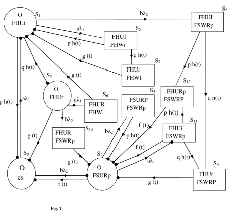
The following are the possible transition states of the system:

S0 = (O, cs), S1 = (O, FHUi), S2 = (O, FSURp),

S3 = (O, FHUr), S4 = (FSURP, FSWRp), S5 = (FHUI, FHWi),

S6 = (FHUR, FHWi), S7 = (FHUr, FHWi),

S8 = (FHUI, FSWRp),S9 = (FHUr, FSWRP),

S10 = (FHUR, FSWRp),

The state S0 – S3, S11 are regenerative states while the states S4

– S10, S12 are non-regenerative as shown in figure 1

3. RELIABILITY INDICES

3.1 Transition Probabilities and Mean

Sojourn Times

Simple probabilistic considerations yield the following

expressions for the non-zero elements











0

(

)

(

q

t

dt

Q

p

_ij _ij _ij by taking all distributions

exponential

i.e. h(t) = 1

1

t

e





, f(t) =



e

t and g(t) =



e

t:

p01= 1

1 2 a a b







, p02= 1 2 2 b a b







, 1 2 1,

1

13

_

_



   b a q p , 1 2 1 1

15

_

_



   b a a p , 1 2 1 1 5 .

11

_

_



   b a pa p , 1 2 1 1 57 .

11

_

_



   b a qa p , 1 2 1 2 12 , 8 .

12

_

_



   b a pb p , 1 2 1 2 89 .

12

_

_



   b a qb p , 2 1

20 _ _ _

    b a p , 1 2 1 2

24

_

_



   b a b p , 1 2 1 1 11 ,

2

_

_



   b a a p , 1 2 1 2 4 .

22

_

_



   b a b p , 2 1 1

36

_

_

(3)

, 2 1 2 10 ,

3

_

_



   b a b p , 2 1 1 6 .

31

_

_



   b a a p , 2 1 2 10 .

32

_

_



   b a b

p

11,2



p

,

p

11,2.9



q

(1) It can be easily verified that

p01+p02=p10+p13+p15+p18=p20+p24+p2,11=p30+p36+p3,10=p11,2+p1 1,9=p10+p13+p11.5+p11.57+p12.8,12+p12.89=p30+p31.6+p32.10=

p11,2+p11,2.9 = 1 (2)

The mean sojourn times (i) is the state Si are

, 1 2 1 0    b a 

 1 ,

1 2 1 1        b a , 1 2 1

2 _ _ _

    b a , 1 2 1

3 _ _ _

    b a , 1 1 11

_



 (3)

Also

0 02 0

m



m





,

m

₁₀



m

₁₃



m

₁₅



m

₁₈





₁,

20 24 2,11 2

m



m



m





,

m

₃₀



m

₃₆



m

_3,10





₃, 11 9 , 11 2 ,

11



m





m

(4)

And

)

(

1 89 . 12 12 , 8 . 12 57 . 11 5 . 11 10

10

m

say

m









1 20 22.4 21.11 2

(

)

m



m



m





say

1 30 36 32.10 3

m



m



m





(say) (5)

For h(t) = 1

1

t

e





, f(t) =



e

t and g(t) =



e

t, we have

(

)

(

)

(

)

1 1 2 1 2 1

1 1

1 1 2 1

a b a b

a b

q a l l a l l qq m

q a l l q

+ + + +

=

+ +

,



1₂

1 



, 1 3

1 





(6)

3.2 Reliability and Mean Time to System

Failure (Mtsf)

Let i(t) be the cdf of first passage time from regenerative

state i to a failed state. Regarding the failed state as absorbing

state, we have the following recursive relations for i(t):

(7)

Where j is an un-failed regenerative state to which the given

regenerative stat I can transit and k is a failed state to which

the state I can transit directly.

Taking LST of above relation (7) and solving for

f



₀

( )

s

We have

R*(s) = 1 0( )s s f

-  ₍₈₎

The reliability of the system model can be obtained by taking

Laplace inverse transform of (8).

The mean time to system failure (MTSF) is given by

MTSF =

s s o s ) ( ~ 1 lim 0



= 1

1 N D

(9)

where

N1 =



₀



p

₀₁



₀



p

₀₂



₂



p p

₀₁ ₁₃



₃

D1 =

1 

p

01



p

10



p p

13 30





p p

02 20

3.3 Steady State Availability

Let Ai(t) be the probability that the system is in up-state at

instant ‘t’ given that the system entered regenerative state i at

t = 0. The recursive relations for Ai(t) are given as

(10) (10)

Where j is any successive regenerative state to which the

regenerative stste I can transit through n≥1 (natural number)

transitions. Mi(t) is the probability that the system is up

initially in state

S

_i



E

is up at time t without visiting to

any other regenerative state, we have

 1 2

0

( )

a b t

M t



e

  ,  1 2

1

( )

a b t

(4)

 1 2

2

( )

a b t

M t



e

  

F t

,  1 2

3

( )

a b t

M t



e

  

G t

(11)

Taking LT of above relations (10) and solving for

A s

₀*

( )

, the steady state availability is given by

* 0( ) lim_s ₀ 0( )

A sA s



  2

2 N D

 (12)

where

N2=p20[p10+p13(p30+p32.10)+p12.8,12+p12.89]



0 +p20p01

(



1



p

13



3

)

+[ p10p02+p13(p02p30+p32.10)+p12.8,16+ p12.89]



2 and

D2=p20[p10+p13(p30+p32.10)+p12.8,16+p12.89]



0+p20p01

(



₁





p

₁₃



₃



)

+ [p10p02+p13(p02p30+p32.10)

+p12.8,16+ p12.89 ] (





2



p

2,11



11



)

3.4 Busy Period Analysis for Server

(a) Due to Hardware Failure

Let BiH(t) be the probability that the server is busy

in repairing the unit due to hardware failure at an instant ‘t’

given that the system entered state i at t = 0. The recursive

relations for BiH(t) are as follows:

(11) (13)

where WiH(t) be the probability that the server is busy in state

Si due to hardware failure upto time t without making any

transition to any other regenerative state or returning to the

same via one or more non-regenerative states and so

 1 2  1 2

1

( )

1

©qh(t)©1

( )

a b t a b

H

W

t



e

 

H t

 



a e



 



_

G t

) ( ) 1 ) ( (

) ( ) 1 ) (

(_b ₂_e(a1 b2)t_qh_t _G_t  _b ₂_e(a1 b2)t_qh_t _F _t



_

 

_

 

 1 2  1 2

3

( )

1

©1

( )

a b t a b

H

W

t



e

 

G t

 



a e



 



_

G t

 1 2

2

©1

( )

a b t

b



e

 

G t





 



)

(

)

(

11

t

H

t

W

H



(12) (14)

(b) Due to replacement of the software

Let

B

_iS(t) be the probability that the server is busy due to replacement of the software at an instant ‘t’ given that the

system entered the regenerative state i at t = 0. We have the

following recursive relations for

B

_iS(t):

(13) (15)

where WiS(t) be the probability that the server is busy in state

Si due to replacement of the software up to time t without

making any transition to any other regenerative state or

returning to the same via one or more non-regenerative states

and so

)

(

)

1 (

)

(

)

(

2 ( )

) ( 2

2 1 2

1

t

F

e

b

t

F

e

t

W

H



ab t





ab t



(14)

Taking LT of above relations (11) and (13) and solving for

* 0

( )

H

B

s

and

B

₀*S

( )

s

, the time for which server is busy due to repair and replacements respectively is given by

*

0 0

0

lim

( )

H H

s

B

sB

s





= 3

2 H

N D

And

*

0 0

0

lim

( )

S S

s

B

sB

s





= 3

2 S

N D

(15) (17)

where

3 01 20 1 13 3 2,11 10 02 12.8,12

12.89 13 30 02 32.10 11

( (0) (0)) (

( ) (0)

H H H

H

N p p W p W p p p p

p p p p p W

   

  

 



3 2,11 10 02 12.8,12 12.89 13 30 02 32.10 2

(

( ) (0)

S

N p p p p p

p p p p W

  

  

and D2 is already mentioned.

3.5 Expected Number Of

Replacements Of The Units

(a) Due to Hardware Failure

Let RiH(t) be the expected number of replacements of the

(5)

the system entered the regenerative state i at t = 0. The

recursive relations for Ri H

(t) are given as

(16) (18)

Where j is any regenerative state to which the given regenerative state I transits and δj =1, if j is the regenerative

state where the server does job a fresh, otherwise δj =0.

(b) Due to Software Failure

Let RiS(t) be the expected number of replacements of the

failed software by the server in (0, t] given that the system entered the regenerative state i at t = 0. The recursive relations for Ri

S

(t) are given as

(17) (19)

state where the server does job a fres

Taking LST of relations (16) and (17). And, solving for

0

( )

H

R



s

and

R s



₀S

( )

. The expected numbers of replacements per unit time to the hardware and software failures are respective of given by

0 0

0

( )

lim

( )

H H

s

R

sR

s



 



₌ 4

2 H

N D

And ₀ ₀

0

( )

lim

( )

S S

s

R

sR s



 



₌ 4

2 S

N D

(18) (20)

where

4

H

N

=p01p20(p10+p12.8,12+p11.5)+p11,2

)

(

10 02 12.8,12 12.89 13 30 02 32.10 11

,

2

p



)

4

S

N

=(p20+p22.4)+ [ p10p02+p13(p02p30+p32.10)+p12.8,16+ p12.89]

and D2 is already mentioned.

3.6 Expected Number of Visits by

The Server

Let Ni(t) be the expected number of visits by the server in (0,

t] given that the system entered the regenerative state i at t = 0. The recursive relations for Ni(t) are given as

(19)

state where the server does job afresh, otherwise δj =0.

Taking LST of relation (19) and solving for

N s



₀

( )

. The expected number of visit per unit time by the server are given by

0 0

0

( ) lim ( )

s

N sN s



   = 5

2

N

D

(20) (22)

where

N5 = p20 [ p10+p13 (p30 +p32.10)+ p12.8,12+ p12.89 ]

and D2 is already specified.

4. PROFIT ANALYSIS

The profit incurred to the system model in steady state can be

obtained as

0 0 1 0 2 0 3 0 4 0 5 0

H S H S

P



K A



K B



K B



K R



K R



K N

(21)

where

K0 = Revenue per unit up-time of the system

K1 = Cost per unit time for which server is busy due to

hardware failure

K2 = Cost per unit time for which server is busy due to

software failure

K3 = Cost per unit replacement of the failed hardware

component

K4 = Cost per unit replacement of the failed software

K5 = Cost per unit visit by the server and

0, 0 , 0 , 0 , 0 , 0

H S H S

A B B R R N are already

defined.

5. PARTICULAR CASE

Suppose g(t) =

a

e

-at, h(t) = 1

1

t

e

q

- , f(t) =

q

e

-qt We can obtain the following results

MTSF (T0) = 1 1 N D

,

Availability (A0) = 2 2 N D

,Busy period due to hardware failure

 

3 0

2 H

H N

B D



Busy period due to software failure

 

3 0

2 S

S

N

B

D

(6)

Expected number of replacements at hardware failure

 

4

0 2 H H N R D 

Expected number of replacements at software failure

 

4 0 2 S S N R D 

Expected number of visits by the server

 

5 0 2 N N D  (24) where







_



_

_

_





1 2

1 1 2

1 2 1 2 1 2 1

1 1 1 2 1

2 a

b

N

a

b

a

b

a

b

a q

a

b

R



 



 



 

 

 

  

 





_





_









_

















_{ }

















 



1 1 2 1 1 2

1 1 2 2 1 2

1 1 1 2 1 2 1

-a

D

a

b

a

b

a

b

a

b

a

b

p a

b

R



 



 

 

 







 



 

















_





_











1 1 2 1 2 1 2 1

1 2

R

a

b

a

b

a

b

a

b



 



 



 



















 





















2 1 2 1 1 1 1 1 2 2 1 1 1 1 2 1 1 1 1

1 2 1 1

D a b p a a a b

a q a b q q

a b R

                                 _   _           _    _















 







1 1 1 1 2

2 1 2

1 2

1 1 1 2 1 2 1

2 p

a

b

N

a

b

q

a

b

a

b

R



 

 

 



 

 



 

 

  







 









_















_







































1 1 1 1 2 1 2

2

1 2 1 1 2 1

1 2 1 2 1 1 2

1 2 1 2

3

1 1 2 1

2

1 1 2 1 2 1 2

H

a

b

a

b

a

b

q

q a

b

q a

b

a

b

a

b

a

b

a

b

N

a

b

a

b

a

b

a

b

   







 



  







 







  

 







































1 1 2



1 2



3

1 2 1 1 2

S a a b b

N

a b a b

 



 

 



 



  



1



4 1 2 H pa N a b



  ,







1 1



2 1 2



4

1 2 1 2 1

S a a b b

N

a b a b

 



 



 

     













1 1 1 1 2 1 1 2

5

1

a q a b a a b

N

R



_

     

  

  



 

 _ 

6. CONCLUSION

In the present study, the numerical results

considering a particular case are obtained to carry out the

profit analysis of a computer system by giving the priority to

repair activities of h/w components over replacement of s/w

components. Using these results, the graphs for mean time to

system failure (MTSF), availability and profit are drawn with respect to h/w failure rate (λ2) for fixed values of other

parameters as shown respectively in figures 2nd,3rd and 4th . From these figures, it is concluded that MTSF deceases with

the increase of h/w and s/w failures rates. However, MTSF

goes on increasing as repair rate (α), replacement rate (θ) of the unit at s/w failure and replacement rate (θ1) of the unit at

h/w failure increase. The results obtained for availability and

profit indicate that the value of these measures decrease with

increase of h/w and s/w failure rate (λ1) and (λ2) respectively.

But their values increase if repair rate (α) and replacement rates (θ) and (θ1) increase.

Thus it is concluded that the concept of priority

given to the replacement and repair of h/w components over

replacement of s/w components is not much economically

beneficial as compare to the system in which no such priority

(7)

[image:7.595.61.514.90.509.2]

State Transition Diagram

Fig. 1

Up-state

Failed state

Regenerative point

FSURP

FSWRp

FHUi

FSWRp

FHURp

FSWRP

FHUR

FSWRp

FHUr

FHWI

FHUI

FHWi

FHUI

FSWRp

O

FHUr

O

cs

O

FHUi

O

FSURp

S

3

S

0

S

₂

S

1

aλ

1

p h(t)

aλ

1

p h(t)

q h(t)

g (t)

S

9

S

10

S

7

S

5

S

4

bλ

2

f (t)

FHUr

FSWRP

bλ

2

S

8

q h(t)

S

12

p h(t)

g (t)

FHUR

FHWi

bλ

2

f (t)

g (t)

S

6

bλ

2

q h(t)

g (t)

S

11

aλ

1

p h(t)

q h(t)

aλ

1

p h(t)

(8)

GRAPH BETWEEN MTSF AND FAILURE RATE

0 20000 40000 60000 80000 100000 120000 140000

0.01 0.02 0.03 0.04 0.05 0.06 0.07 0.08 0.09

FAILURE RATE (λ1)

M

T

S

F

a=0.3,b=0.7,λ2=0.005,θ=20,

θ1=10,p=0.3,q=0.7,α=2.5 a=0.7,b=0.3,λ2=0.02,θ=20,

θ1=10,p=0.3,q=0.7,α=2.5 a=0.7,b=0.3,λ2=0.005,θ=30,

θ1=10,p=0.3,q=0.7,α=2.5 a=0.7,b=0.3,λ2=0.005,θ=20, θ1=20,p=0.3,q=0.7,α=2.5

a=0.7,b=0.3,λ2=0.005,θ=20, θ1=10,p=0.3,q=0.7,α=2.5

a=0.7,b=0.3,λ2=0.005,θ=20, θ1=10,p=0.7,q=0.3,α=2.5 a=0.7,b=0.3,λ2=0.005,θ=20,

θ1=10,p=0.3,q=0.7,α=3.5

GRAPH BETWEEN FAILURE RATE AND AVAILABILITY

0.999 0.9992 0.9994 0.9996 0.9998 1 1.0002

0.01 0.02 0.03 0.04 0.05 0.06 0.07 0.08 0.09

A

V

A

IL

A

B

IL

IT

Y

a=0.3,b=0.7,λ2=0.005,θ=20, θ1=10,p=0.3,q=0.7,α=2.5

a=0.7,b=0.3,λ2=0.02,θ=20, θ1=10,p=0.3,q=0.7,α=2.5

a=0.7,b=0.3,λ2=0.005,θ=20,

θ1=10,p=0.7,q=0.3,α=2.5

a=0.7,b=0.3,λ2=0.005,θ=20, θ1=10,p=0.3,q=0.7,α=3.5

a=0.7,b=0.3,λ2=0.005,θ=20, θ1=20,p=0.3,q=0.7,α=2.5

a=0.7,b=0.3,λ2=0.005,θ=30, θ1=10,p=0.3,q=0.7,α=3.5

a=0.7,b=0.3,λ2=0.005,θ=20, θ1=10,p=0.3,q=0.7,α=2.5

GRAPH BETWEEN FAILURE RATE AND PROFIT

14900 14910 14920 14930 14940 14950 14960 14970 14980 14990 15000

0.01 0.02 0.03 0.04 0.05 0.06 0.07 0.08 0.09

P

R

O

F

IT

a=0.7,b=0.3,λ2=0.005,θ=20, θ1=10,p=0.3,q=0.7,α=2.5

a=0.7,b=0.3,λ2=0.02,θ=20, θ1=10,p=0.3,q=0.7,α=2.5

a=0.7,b=0.3,λ2=0.005,θ=20,

θ1=10,p=0.7,q=0.3,α=2.5 a=0.7,b=0.3,λ2=0.005,θ=30,

θ1=10,p=0.3,q=0.7,α=2.5

a=0.7,b=0.3,λ2=0.005,θ=20, θ1=20,p=0.3,q=0.7,α=2.5 a=0.3,b=0.7,λ2=0.005,θ=20,

θ1=10,p=0.3,q=0.7,α=2.5

a=0.7,b=0.3,λ2=0.005,θ=20,

θ1=10,p=0.3,q=0.7,α=3.5

Fig.3

(9)

7. REFERENCES

[1] Friedman, M.A. and Tran, P. 1992: Reliability Techniques for Combined Hardware / Software Systems. Proceedings of Annual Reliability and Maintainability Symposium, pp. 209-293.

[2] Welke, S.R.; Johnson, B.W. and Aylar, J.H. 1995: Reliability Modeling of Hardware Software Systems. IEEE Transactions on Reliability, Vol. 44(3), pp. 413-418

[3] Malik, S.C. and Anand, Jyoti 2010: Reliability And Economic Analysis of a Computer System With Independent H/W and S/W Failures. Bulletin of Pure and Applied Sciences (BPASS), Vol.29E(No.1),pp.141-153

[4] Malik, S.C. and Anand, Jyoti 2011: Reliability Modeling of a Computer System With Priority for Replacement at Software Failure over Repair Activities at H/W Failure.

International Journal of Statistics and System (IJSS), ISSN 0973-2675, Vol. 6(3),pp.315-325.

[5] Malik, S. C. and Ashish Kumar 2011. Profit Analysis of a Computer System with Priority to Software Replacement over Hardware Repair Subject to Maximum Operation and Repair Times, International Journal of Engineering Science & Technology, Vol.3, No. 10, pp. 7452- 7468.

[6] Lai, C.D.; Xie, M.; Poh, K.L.; Dai, Y.S. and Yang, P. 2002: A model for availability analysis of distributed software / hardware systems, Information and Software Technology, Vol. 44, pp. 343-350.