Learning in Neural Spatial Interaction Models: A Statistical Perspective

Munich Personal RePEc Archive

Learning in Neural Spatial Interaction

Models: A Statistical Perspective

Fischer, Manfred M.

Vienna University of Economics and Business

2002

Online at

https://mpra.ub.uni-muenchen.de/77788/

Learning in Neural Spatial Interaction Models:

A Statistical Perspective*

Manfred M. Fischer

Department of Economic Geography & Geoinformatics

Vienna University of Economics and Business Administration

Rossauer Laende 23/1, A-1090 Vienna, Austria

Email: [email protected]

* The author gratefully thanks Martin Reismann (Department of Economic Geography

Abstract. In this paper we view learning as an unconstrained non-linear minimization problem in which the objective function is defined by the negative log-likelihood

function and the search space by the parameter space of an origin constrained product

unit neural spatial interaction model. We consider Alopex based global search, as

opposed to local search based upon backpropagation of gradient descents, each in

combination with the bootstrapping pairs approach to solve the maximum likelihood

learning problem. Interregional telecommunication traffic flow data from Austria are

used as test bed for comparing the performance of the two learning procedures. The

study illustrates the superiority of Alopex based global search, measured in terms of

Kullback and Leibler’s information criterion.

Key Words: Maximum likelihood learning, local search, global search, backpropagation

of gradient descents, Alopex procedure, origin constrained neural spatial interaction

1 Introduction

In many spatial interaction contexts, little is known about the form of the spatial

interaction function that is to be approximated. In such cases it is not possible to utilize

a parametric modeling approach where a mathematical model is specified with

unknown coefficients that have to be estimated. Neural spatial interaction models

relieve the model user of the need to specify exactly a model that includes all necessary

terms to model the true spatial interaction function. Two major issues have to be solved

when applying a neural spatial interaction model in a real world context: first the

representation problem, and, second the learning problem. Our interest centers at the

latter problem.

This contribution departs from earlier studies in neural spatial interaction modeling in

three respects. First, current research generally suffers from least squares and Gaussian

assumptions that ignore the true integer nature of the flows and approximate a

discrete-valued process by an almost certainly misrepresentative distribution. To overcome this

deficiency we adopt a more suitable approach for solving the learning problem, namely

maximum likelihood learning [estimation] under more realistic distributional

assumptions of Poisson processes. Second, classical [i.e. unconstrained summation unit]

neural spatial interaction models represent – no doubt – a rich and flexible class of

spatial interaction function approximators to predict flows, but may be of little practical

value if a priori information is available on accounting constraints on the predicted

flows. We focus attention on the only existing generic neural network model for the

case of spatial interaction. Third, we utilize the bootstrapping pairs approach with

replacement to overcome the generally neglected issue of fixed data splitting and to get

a better statistical picture of the learning and generalization variability of the model

concerned.

Succinctly put, the objective of the paper is twofold. First, we develop a rationale for

specifying the maximum likelihood learning problem in product unit neural networks

for modeling origin constrained spatial interaction flows as recently introduced in

Fischer, Reismann and Hlavackova-Schindler (2002). Second, we consider Alopex

in combination with the bootstrapping pairs approach to solve the maximum likelihood

learning problem.

The paper proceeds as follows. The next section sets forth the context in which the

learning problem is considered. Section 3 views learning as an unconstrained non-linear

minimization problem in which the objective function is defined by the negative

log-likelihood and the search space by the parameter space. In the sections that follow we

discuss details how the highly non-linear learning problem can be solved. We consider

two learning procedures in some more detail: gradient descent based local search [the

most widely used technique in unconstrained neural spatial interaction modeling] in

Section 4 and Alopex based global search in Section 5. Section 6 serves to illustrate the

application of these procedures in combination with the bootstrapping pairs approach to

address the issue of network learning. Interregional telecommunication traffic flow data

are utilized as test bed for evaluating the two competing learning approaches. The

robustness of the procedures is measured in terms of Kullback and Leibler’s

information criterion. Section 7 outlines some directions for future research.

2 The Context

Before discussing the learning problem we must specify the context in which we

consider learning. Our attention is focused on learning in origin constrained product

unit neural spatial interaction models. Throughout the paper we will be concerned with

the data generated according to the following conditions.

Assumption A: Observed data are the realization of the sequence

(

)

{

Z_u = X Y_u, _u ,u=1,...,U

}

of

(

N+ ×1

)

1 independent vectors

(

N∈฀

)

defined as a Poisson probability space.

The random variables Yu represent targets. Their relationship to the variables Xu is of

primary interest. When E Y

( )

_u < ∞, the conditional expectation of Y_u given X_u exists, denoted as g=E Y X

(

u u

)

. Defining εu ≡Yu −g X

( )

u

( )

u u u

The unknown spatial interaction function g embodies the systematic part of the

stochastic relation between Y_u and X_u. The error ε_u is noise, with the property

(

u u

)

0

E ε X = by construction. Our problem is to learn the mapping g from a

realization of the sequence

{ }

Z_u .

We are interested in learning the mapping g for the case of origin constrained spatial

interaction. Because g is unknown, we approximate it using a family of known

functions. Of particular interest to us are the output functions of origin constrained

product unit neural spatial interaction models as recently introduced in Fischer,

Reismann and Hlavackova-Schindler (2002).

Assumption B: Model output is given by

(

)

2

1 2 1

, hn

j H

H

j h h n j

h n j

xβ

Ω ψ γ j

= = −

  

= _  _

 



∑

∏



x w (2)

for j=1,...,J with j ψh, h:฀ →฀ , and

2J

x∈฀ , that is x = (x1, x2,…, x2j-1,..., x2J-1, x2J)

where x_2j−1 represents a variable pertaining to destination j

(

j=1,...,J

)

and x_2j a variable characterizing the separation from region i to region j

(

i=1,..., ;I j=1,...,J

)

of the spatial interaction system under scrutiny. β_hn

(

h=1,...,H n; =2j−1, 2j

)

are the input-to-hidden connection weights, and γh

(

h=1,...,H

)

the hidden-to-output weights

in the j-th module of the network model. The symbol w is a convenient shorthand

notation of the (3H)-dimensional vector of all the model parameters. ψj

(

j=1,...,J

)

represents a non-linear summation unit and j_h

(

h=1,...,H

)

a linear hidden product unit transfer function. The model output function is explicitly indexed by the number,

H, of hidden units in order to indicate the dependence. Finally, it is worth noting that

models of type (2) utilize a product unit rather than the generally used standard

summation unit neural network framework for modeling interactions over space. The

product units compute the product of inputs, each raised to a variable power.

A leading case that is considered in this paper occurs when jh

( )

⋅ is specified as

Bradley-Terry-Luce model augmented by a bias unit b_{( )i} to build the a priori information into the model structure (for a mathematical derivation see Fischer,

Reismann and Hlavackova-Schindler, 2002):

(

)

_{( )}

2 1 2 1

2 1 1 2 1

, 1, ...,

hn

h n

j H

h n h n j H

i J H j j

h n j h n j

x

b j J

x β β γ Ω γ = = − = = = − =

∑ ∏

=

∑∑ ∏

 x w ' ' ' ' ' ' (3)

for j=1,...,J. b_{( )i} is the bias signal generated by a dummy unit whose output is clamped at the scalar t_i⋅, where t_i⋅ denotes the observed flow from region i to each of the J regions.

3 The Learning Problem

If we view (3) as generating a family of approximations – as w ranges over W, say – to

a spatial interaction function g, then we need a way to pick the best approximation from

this family. This is the function of network learning (also termed training or parameter

estimation). It is convenient to consider learning as an unconstrained non-linear

minimization problem in which the objective function is defined by a loss (error, cost)

function and the search space by the (3H)-dimensional parameter space. Formally,

( )

min

W

∈ λ

w w (4)

where λ

( )

w represents the loss function measuring the network performance given the parameter w and observation z=

(

x y,

)

. It is evident that the choice of the loss function plays a crucial role in the determination of the optimal parameter ˆw. We follow Fischer

and Reismann (2002b) to specify an appropriate loss function. Hereby, we assume that

the objective is to find that neural spatial interaction model which is the most likely

explanation of the observed data set (Rumelhart et al., 1995). We express this as

( )

(

)

P M

(

( )

_{( )}

)

P

(

H

( )

)

P M

P M

H

H Ω Ω

Ω w = w w (5)

where P M

(

ΩH

( )

w

)

is the probability that model ΩH

( )

w would have produced the observed data M. P

(

ΩH

( )

w

)

represents the unconditional probability density of

( )

H

Ω w and P M

( )

that of M.

Since sums are easier to work with than products, we will maximize the log of

( )

(

)

P ΩH w M , and since this log is a monotonic transformation, maximizing the log

is equivalent to maximizing the probability itself. In this case we get

( )

(

)

(

( )

)

(

( )

)

( )

lnP ΩH w M =lnP M ΩH w +lnP ΩH w −lnP M (6)

The probabilityP M

( )

of the data is not dependent on ΩH

( )

w . Thus, it is sufficient to maximize the first two terms of the right hand side of Equation (6). The first of these

terms represents the probability of the data given the model, and hence measures how

well the network accounts for the data. The second term is a representation of the model

itself; that is, it is a prior probability of the model that can be utilized to get information

and constraints into the learning procedure.

We focus solely on the first term, the performance, and begin by noting that the data

can be broken down into a set of observations, M =

{

z_u =

(

x y_u, _u

)

u=1,...,U

}

, each z_u, we will assume chosen independently of the others. Hence we can write the probability

of the data given the model as

( )

(

)

(

( )

)

(

( )

)

ln ln _u ln _u

u u

P M ΩH w =

∏

P z ΩH w =

∑

P z ΩH w (7)

Note that this assumption permits to express the probability of the data given the model

as the sum of terms, each term representing the probability of a single observation

given the model. We can still take another step and break the data into two parts: the

( )

(

)

(

( )

)

( )

ln ln _{u u} and ln _u

u

u u

P M ΩH w =

∑

P y x P xΩH w +

∑

(8)

Since we assume that xu does not depend on the model, the second term of Equation

(8) will not affect the determination of the optimal model. Thus, we need only to

maximize the first term of the right-hand side of Equation (8).

Up to now we have – in effect – made only the assumption of the independence of the

observed data. To proceed further, we have to specify the form of the distribution of

which the model output is the mean. In line with Assumption A that the observed data

are the realization of a sequence of independent Poisson random variables we can write

the probability of the data given the model as

( )

(

and

)

( )

exp

(

( )

)

!

u

y

u u

u

u u u

u

P y x

y H H H Ω Ω Ω − =

∏

w w w (9)

and, hence, define a maximum likelihood estimator as the parameter that maximizes the

log-likelihood function

( )

(

( )

( )

)

max max uln _{u u}

u

L y ΩH ΩH

∈ = ∈

∑

−

w W w w W w w

(10)

Instead of maximizing the log-likelihood it is more convenient to minimize the negative

log-likelihood function λ

( )

w

( )

( )

( )

min min _uln H _u H _u

uy Ω Ω

∈ λ = ∈ −

∑

− 

w W w w W w w (11)

The function λ is called the loss, cost or objective function. w is a (3H)-dimensional

vector called the design vector. The point ˆw is a global minimizer for λ

( )

w if

( )

wˆ ≤

( )

w

λ λ for all ∈ 3H

฀

w . A parameter vector ˆw is a strict local minimizer of

( )

w

( )

2

ˆ 0

T ∇ >

w λ w ]. λ is typically a highly non-linear function of the parameters. As a

consequence, it is in general not possible to find closed-form solutions for the minima.

In the sections that follow we discuss how the learning problem (11) can be solved. We

seek a solution to what is typically a highly non-linear optimization problem. We first

consider the gradient descent based search and then the Alopex based global search

procedures.

4 Gradient Descent Based Search

The most prominent procedures solving the learning problem (11) are gradient descent

techniques. These methods transform the minimization problem into an associated

system of first-order ordinary differential equations which can be written in compact

matrix form (see Cichocki and Unbehauen, 1993) as

(

,

)

_w

( )

d

s

d = − ∇

w

w w

s µ λ (12)

with

3 1_{, ...,}

T H

dw

d dw

d ds ds

 

= _ _

w

s (13)

( )

w

∇ λ w represents the gradient operator of λ

( )

w with respect to the (3H )-dimensional parameter vector w. µ

(

w,s

)

denotes a 3H×3H positive definite symmetric matrix with entries depend on time s and the vector w

( )

s .

In order to find the desired vector ˆw that minimizes the loss function λ

( )

w we need to solve the system of ordinary equations (12) with initial conditions. Thus, the minima of

( )

w

λ are determined by the following trajectory of the gradient system with

( )

ˆ lim

s→∞ s

=

But it is important to note that we are concerned only with finding the limit rather that

determining a detailed picture of the whole trajectory w

( )

s itself. In order to illustrate that the system of differential equations given by (12) is stable let us determine the time

derivative of the loss function

( )

(

)

( )

3 1

0

H

T k

w w

k k

d

,s

ds = s

∂ ∂

= = − ∇_ _ ∇ ≤

∂ ∂

∑

w

w w w

w

λ λ _{λ µ λ}

(15)

under the condition that the matrix µ

(

w,s

)

is symmetric and positive definite. Relation (15) guarantees under appropriate regularity conditions that the loss function decreases

in time and converges to a stable local minimum as s→ ∞. When dw/ds=0 then this

implies ∇λ

( )

w =0 for the system of differential equations. Thus, the stable point coincides either with the minimum or with the inflection point of the loss function (see

Cichocki and Unbehauen, 1993).

The speed of convergence to the minimum depends on the choice of the entries of

(

w,s

)

µ . Different choices for µ implement different specific gradient based search

procedures: In the simplest and most popular procedure, known as gradient descent, the

matrix µ

(

w,s

)

is reduced to the unity matrix multiplied by a positive constant η that is called the learning parameter. It is interesting to note that the vectors dw/ds and

( )

∇λ w are opposite vectors. Hence, the time evaluation of w

( )

s will result in the minimization of λ

( )

w as time s goes on. The trajectory w

( )

s moves along the direction which has the sharpest rate of decrease and is called the direction of steepest

descent.

The discrete-time version of the steepest descent [also termed gradient] procedure can

be written in vector form as

(

s+ =1

)

( ) ( )

s −η s ∇_w

(

( )

s

)

w w λ w (16)

that the sometimes extreme local irregularity ('_roughness'_, '_ruggedness'_{) of the function}

λ over W arising in neural spatial interaction models may require the development and

use of appropriate modifications of the standard procedure given by (16).

We utilize the simplest version of (16), that is, η

( )

s =η [η sufficiently small] in combination with the technique of backpropagation popularized in a paper by

Rumelhart, Hinton and Williams (1986) for evaluating the derivatives of the loss

function with respect to the parameters. This technique provides a computationally

efficient method for evaluating such derivatives. It corresponds to a propagation of

errors backwards through the spatial interaction network. Because of the relative

familiarity of this evaluation technique we do not go into details regarding the specifics

of implementation. Those not familiar with backpropagation are referred to Bishop

(1995) for further information.

5 Alopex-Based Global Search

Although computationally efficient, gradient based minimization procedures, such as

backpropagation of gradient errors, may lead only to local minima of λ

( )

w that happen to be close to the initial search point w

( )

0 . As a consequence, the quality of the final solution of the learning problem is highly dependent on the selection of the initial

condition. Global search procedures are expected to lead to optimal or '_near-optimal'

parameter configurations by allowing the network model to escape from local minima

during training. Genetic algorithms and the Alopex procedure are attractive candidates.

We utilize the latter as described in Fischer and Reismann (2002b).

The success of global search procedures in finding a global minimum of a given

function such as λ

( )

w over w ∈ W hinges on the balance between an exploration process, a guidance process and a convergence-inducing process (see Hassoun, 1995).

The exploration process gives the search a mechanism for sampling a sufficiently

diverse set of parameters w in W. The Alopex procedure performs an exploration

process that is stochastic in nature. The guidance process is an implicit process that

evaluates the relative quality of search points and utilizes correlation guidance to move

solution ˆw. The convergence-inducing process is realized effectively by a parameter T,

called temperature in analogy to the simulated annealing procedure, that is gradually

decreased over time. The dynamic interaction among these three processes is

responsible for giving the Alopex search procedure its global optimizing character.

Alopex is a correlation-based method for solving the learning problem (see Bia, 2000;

Unnikrishnan and Venugopal, 1994; Harth and Pandya, 1988). The loss function λ is

minimized by means of weight changes that are calculated for the s-th step (s>2) of

the iteration process as follows:

( )

(

1

)

sgn

(

( )

)

k k k

w s =w s− +δ s −p s (17)

where δ is the step size that has to be chosen a priori, and s is an uniformly

distributed random value with s∈

[ ]

0,1 . The probability of change of the parameter is

calculated as

( )

(

(

( ) ( )

)

)

1

1 exp /

k k

p s = + C s T s − (18)

with C_k

( )

s given by the correlation

( )

k

C s =wk

(

s− −1

)

wk

(

s−2

)

 λ

(

wk

(

s−1

)

)

−λ

(

wk

(

s−2

)

)

 (19)

( )

(

( )

)

k k

w s w s

= ∆ ∆λ

The weight will be incremented in a given fixed magnitude δ , when ∆w_k

( )

s >0, and the opposite when it is less than zero. The sign of C_k indicates whether λ varies in the same way as w_k. If C_k >0, both λ and w_k will be raised or lowered. If C_k <0, one will be lowered and the other one raised. If T is too small, the algorithm gets trapped

( )

( )

(

)

1

if is a multiple of 3

1 otherwise

s k k s S

C s s S

HS T s

T s

δ −

= − 

 = 

 ₋



∑ ∑

s'

'

(20)

where 3H denotes the number of parameters. The annealing schedule controls the

randomness of the algorithm. When T is small, the probability of changing the

parameter is around zero if C_k is negative and around one if C_k is positive.

If T is large, then pk ≅0.5. This means that there is the same probability to increment or decrement the weights and that the direction of the steps is now random. In other

words, high values of T imply a random walk, while low values cause a better

correlation guidance (see Bia, 2000). The effectiveness of Alopex in locating global

minima and its speed of convergence critically depend on the balance of the size of the

feedback term ∆w_k ∆λ and the temperature T. If T is very large compared to ∆w_k ∆λ

the process does not converge. If T is too small, a premature convergence to a local

minimum might occur.

The algorithm has three control parameters: the initial temperature T, the number of

iterations S over which the correlations are averaged for annealing, and the step size δ .

Setting the temperature high initially, say T =1, 000, one may escape from local

minima. The temperature is lowered at an appropriate rate so as to control the

probability of jumping away from relatively good minima. The correlations need to be

averaged over a sufficiently large number of iterations so that the annealing does not

freeze the algorithm at local minima. S =10 has been found to be appropriate. δ is a

critical control parameter that has to be chosen with care.

It is worth noting that Alopex based global search is similar to the method of simulated

annealing (see Kirkpatrick, Gelatt and Vecchi, 1983), but differs in three important

aspects: first, the correlation

(

∆ ∆λ w

)

is used instead of the change in error ∆λ for parameter updates; second, all parameter changes are accepted at every iteration step;

6 Experimental Environment and Performance Tests

To analyze the performance of the learning procedures discussed in the previous

sections in a real world context we utilize the interregional telecommunication traffic

flow data from Austria as test bed.

The Data Set

The data set was constructed from three data sources: a

(

32, 32 - interregional flow

)

matrix

( )

tij , a

(

32, 32 -distance matrix

)

( )

dij , and gross regional products gj for the 32

telecommunication regions. It contains 992 3-tuples

(

g d t_i, _ij, _ij

)

where the first two components represent the input variables x2j−1 and x2j of the j-th module of the

network model, and the last component the target output. Input data were preprocessed

to lie in [0.1, 0.9]. The telecommunication data stem from network measurements of

carried telecommunication traffic in Austria in 1991, in terms of erlang, which is

defined as the number of phone calls (including facsimile transmissions) multiplied by

the average length of the call (transfer) divided by the duration of the measurement.

Data Splitting, Bootstrapping and Performance Measure

The main goal of network learning is to minimize λ

( )

w while ensuring good model generalization. Thus, we monitor model performance during training to assure that

further learning improves generalization as well as reduces the loss function λ. For this

purpose an additional set of internal validation data, independent from the training data,

is used. In our implementation of the learning procedures network learning will be

stopped when κ =40, 000 consecutive iterations are unsuccessful. κ has been chosen

so large at the expense of the greater training time, to ensure more reliable estimates. Of

course, setting the number of unsuccessful iterations to 40,000 (or more) does not

guarantee that there would be any successful steps ahead if training continued. At some

stage a learning algorithm may recover from some local attractor and accomplish

further error minimization, but we require it should occur within a certain number of

One of the simplest methods for assessing the learning and generalization abilities of a

model is, thus, data splitting. This method simulates learning and generalization by

partitioning the total data set M =

{

(

x y_u, _u

)

,u=1,...,U

}

into three separate subsets: the training set M1=

{

(

xu1,yu1

)

, 1 1,...,u = U1

}

, the internal validation set

(

)

{

}

2 u2, u2 , 2 1,..., 2

M = x y u = U and the test set M₃ =

{

(

x_u3,y_u3

)

, 3 1,...,u = U₃

}

. M₁ is used for learning only, M2 for stopping the learning process and M3 for measuring the

generalization performance. In our study U₁=496,U₂ =U₃ =248.

It is common practice to use random splits of the data. The simplicity of this approach

is appealing. But recent experience has found this approach to be more sensitive to the

specific splitting of the data (see Fischer and Reismann, 2002a). In order to overcome

this problem we use the learning algorithms in combination with the bootstrapping pairs

approach with replacement

[

B=60

]

(see Efron, 1982) to address the issue of network

learning. This approach combines the purity of splitting the data into three disjoint data

sets with the power of a resampling procedure and, thus, allows to get a better statistical

picture of both the learning and prediction variability.

Performance is measured in terms of Kullback and Leibler’s information criterion (see

Kullback and Leibler, 1951), that reflects the conditions under which ML learning is to

be evaluated

( )

(

)

(

)

1 ' ' 1 1 1 ' _'

' 1 _{' 1}

ln , , U u u U u u U _U u

u _{u u}

u _u

y y

y KLIC M

y _ΩH _{x Ω}H _x − = − = = ₌  _{ }   _{ }      = _{ }    _{ }       

∑

∑

∑

w

_∑

w

(21)

where

(

x y_u, _u

)

denotes the u-th pattern of the data set M. The performance measure has

a minimum at zero and a maximum at positive infinity when y_u >0 and

(

x ,_u

)

0 H

Ω w = for any

(

x y_u, _u

)

-pair.

Performance Tests

point in both cases. The solutions to the learning problem may vary as the initial

parameter settings are changed. Despite recent progress in finding the most appropriate

parameter initialization to determine near optimal solutions, the most widely adopted

approach still uses random parameter initialization. In our experiments random

numbers were generated from [-0.3, 0.3] using the rand_uni function from Press et al.

(1992). The order of the input data presentation was kept constant for each run to

eliminate its effect on the result.

For concreteness, we consider the learning problem in a series of increasingly complex

neural spatial interaction models {ΩH

(

x w,

)

, H = 2, 4, 6, 8, 10, 12 ,14} permitting the complexity of the product unit neural network to grow at an appropriate rate. Statistical

theory may provide guidance in choosing the control parameters of the learning

algorithms for optimal tracking, but this is a difficult area for future research. In this

study the Alopex parameters T and S were set to 1,000 and 10, respectively. In order to

do justice to each learning procedure, the critical Alopex control parameter δ [step

size] and the critical gradient descent control parameter η [learning rate] were

systematically sought for each ΩH . Extensive computational experiments with

η ∈{0.0000025, 0.0000050, 0.0000100, 0.0000250, 0.0000500, 0.0001000,

0.0002500} and δ ∈{0.0005, 0.0010, 0.0025, 0.0050, 0.0075, 0.0100, 0.0250, 0.0500,

0.1000} have been performed on DEC Alpha 375 MHz to address the issue of learning

in the above models.

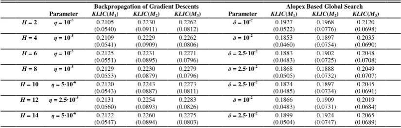
POSITION TABLE 1 ABOUT HERE

Table 1 shows the best solutions of both procedures for ΩH with H = 2, 4, 6, 8, 10, 12

and 14. Learning [in-sample] performance is measured in terms of KLIC M

( )

1 ,

validation performance in terms of KLIC M

( )

₂ and generalization [out-of-sample] performance in terms of KLIC M

( )

3 . The performance values represent the mean of

60

B= bootstrap replications, standard deviations are given in brackets. The results

achieved illustrate that Alopex based global search outperforms backpropagation of

gradient descents in all cases, in terms of both learning and generalization performance.

There is also strong evidence of the robustness of the algorithm, measured in terms of

standard deviation. We attribute Alopex superiority in finding better local minima to its

7 Conclusions and Outlook

Learning neural spatial interaction parameters is like solving an unconstrained

continuous non-linear minimization problem. The task is to find parameter assignments

that minimize the given negative log-likelihood function. Product unit neural spatial

interaction network learning is a multimodal non-linear minimization problem with

many local minima. Local minimization algorithms such as backpropagation of

gradient descents have difficulties when the surface of the search space is flat [that is,

gradient close to zero], or when the surface is very rugged. When the surface is rugged,

a local search from a random starting point generally converges to a local minimum

close to the initial point and to a worse solution than the global minimum.

Global search procedures such as Alopex based search, as opposed to local search, have

to be used in learning problems where reaching the global optimum is at premium. But

the price one pays for using global search procedures in general and Alopex search in

particular is increased computational requirements. The intrinsic slowness of global

search procedures is mainly due to the slow but crucial exploration process employed.

An important lesson from the results of the study and an interesting avenue for research

is, thus, to make global search more speed efficient. This may motivate the

development of a hybrid procedure that uses global search to identify regions of the

parameter space containing promising local minima and gradient information to

References

Bia, A. (2000): A study of possible improvements to the Alopex training algorithm,

Proceedings of the VIth Brazilian Symposium on Neural Networks, pp. 125-130.

IEEE Computer Society Press

Bishop, C.M. (1995): Neural networks for pattern recognition. Clarendon Press,

Oxford.

Cichocki, A. and Unbehauen, R. (1993): Neural networks for optimization and signal

processing. John Wiley, Chichester.

Efron, B. (1982): The jackknife, the bootstrap and other resampling plans. Society for

Industrial and Applied Mathematics, Philadelphia

Fischer, M.M. and Reismann, M. (2002a): Evaluating neural spatial interaction

modelling by bootstrapping, Networks and Spatial Economics [in press]

Fischer, M.M., and Reismann, M. (2002b): A methodology for neural spatial

interaction modeling, Geographical Analysis 34(2) [in press]

Fischer, M.M., Reismann, M. and Hlavackova-Schindler, K. (2002): Neural network

modelling of constrained spatial interaction flows: Design, estimation and

performance issues, Journal of Regional Science 42 [in press]

Harth, E. and Pandya, A.S. (1988): Dynamics of ALOPEX process: Application to

optimization problems. In Ricciardi, L.M. (ed.): Biomathematics and related

computational problems, pp. 459-471. Kluwer, Dortrecht.

Hassoun, M.M. (1995): Fundamentals of neural networks. MIT Press, Cambridge and

London.

Kirkpatrick, S., Gelatt, C.D. and Vecchi, M.P. (1983): Optimization by simulated

annealing, Science 20, 671-680.

Kullback, S. and Leibler, R.A. (1951): On information and sufficiency, Annals of

Mathematical Statistics 22, 78-86

Press, W.H., Teukolsky, S.A., Vetterling, W.T. and Flannery, B.P. (1992): Numerical

recipes in C: The art of scientific computing. Cambridge University Press,

Rumelhart, D.E., Hinton, G.E. and Williams, R.J. (1986): Learning internal

representations by error propagation. In Rumelhart, D.E., McClelland, J.L. and the

PDP Research Group (eds.): Parallel distributed processing: Explorations in the

microstructure of cognition, pp. 318-362. MIT Press, Cambridge [MA]

Rumelhart, D.E., Durbin, R., Golden, R. and Chauvin Y. (1995): Backpropagation: The

basic theory. In Chauvin, Y. and Rumelhart, D.E. (eds.): Backpropagation: Theory,

architectures and applications, pp. 1-34. Lawrence Erlbaum Associates, Hillsdale

[NJ]

Unnikrishnan, K.P. and Venugopal, K.P. (1994): Alopex: A correlation-based learning

algorithm for feedforward and recurrent neural networks, Neural Computation 6,

[image:21.595.84.497.147.279.2]

Table 1.

Approximation to the Spatial Interaction Function Using Backpropagation of Gradient Descents versus Alopex Based Global Search.

Backpropagation of Gradient Descents Alopex Based Global Search Parameter KLIC(M1) KLIC(M2) KLIC(M3) Parameter KLIC(M1) KLIC(M2) KLIC(M3)

H = 2 η = 10-5

0.2105 0.2230 0.2262 δ = 10-2

0.1927 0.1968 0.2120 (0.0540) (0.0911) (0.0812) (0.0522) (0.0776) (0.0698)

H = 4 η = 10-5

0.2109 0.2229 0.2262 δ = 10-2

0.1853 0.1897 0.2035 (0.0541) (0.0909) (0.0806) (0.0460) (0.0754) (0.0690)

H = 6 η = 10-5

0.2125 0.2231 0.2271 δ = 2.5·10-2

0.1883 0.1902 0.2048 (0.0551) (0.0895) (0.0796) (0.0483) (0.0725) (0.0708)

H = 8 η = 10-5

0.2129 0.2230 0.2279 δ = 2.5·10-2

0.1868 0.1888 0.2049 (0.0553) (0.0879) (0.0796) (0.0505) (0.0732) (0.0707)

H = 10 η = 5·10-6

0.2120 0.2243 0.2273 δ = 2.5·10-2

0.1874 0.1897 0.2045 (0.0543) (0.0887) (0.0811) (0.0485) (0.0734) (0.0691)

H = 12 η = 2.5·10-5

0.2131 0.2254 0.2283 δ = 10-2

0.1866 0.1909 0.2019 (0.0560) (0.0893) (0.0826) (0.0483) (0.0731) (0.0684)

H = 14 η = 5·10-6

0.2122 0.2260 0.2275 δ = 2.5·10-2

0.1899 0.1924 0.2065 (0.0547) (0.0894) (0.0803) (0.0504) (0.0747) (0.0689)

Note: KLIC-performance values represent the mean (standard deviation in brackets) of B = 60 bootstrap replications differing in both the initial parameter values randomly chosen from [-0.3; 0.3] and the data split. KLIC(M1): Learning performance measured in terms of average KLIC;KLIC(M2): Validation performance

measured in terms of average KLIC;KLIC(M3): Generalization performance measured in terms of average