Visual Perception based Motion Planning of Mobile Robot using Road Sign

(1)

Visual Perception based Motion Planning of Mobile

Robot using Road Sign

Pradipta K.Das

DRIEMS Cuttack-754022, India

S. C. Mandhata

H.S Behera

VSSUT, Burla-768018 Odisha, India

S.N. Patro

ABSTRACT

In this paper a new method of road map based navigation is proposed. A vision based motion planning of a mobile robot is implemented in a predefined road map. Road map is build with the left and right lane at the junction constructed with 90 degree with respect to the main lane. In our realization the robot moves towards a junction and at each junction takes a photograph of the road sign map and an image matching algorithm is performed at the host machine to compare the captured image with the map stored in the memory and decide the next course of action.

Keywords

Road sign, image matching, Hopfield Neural Network, Hausdorff Distance, Chaos Optimizing, motion planning, Khepera II

1. INTRODUCTION

A basic motion planning problem is to produce a continuous motion that connects a start configuration S and a goal configuration G, while avoiding collision with obstacles. The robot and obstacle geometry is described in a 2D or 3D workspace, while the motion is represented as a path. Different approaches for motion planning can be found in the literatures. In [1], the authors have presented a vision based approach to detect, localize and track stationary masts located near road and intersection borders around a driving vehicle. The approach is based on knowledge about the lane structure of the road which has been extracted by an automatically generated road model. However motion planning is not considered in this paper. The authors in [2] consider a computer vision based system for real-time robust traffic sign detection, tracking, and recognition. The detection is based on the color information and shape of the object. But this approach is prone to error and also motion planning is not considered. In [6]-[7] color based object detection and tracking were studied extensively but like [2] motion planning was not considered. The authors in [8] proposed a vision based motion planning for an autonomous motorcycle. The invariant recognition of broken rectangular biscuits is proposed using fuzzy membership-distance products, called fuzzy moment descriptors [14].

In this paper, we are proposing a vision based motion planning of a mobile robot using road sign detection. In this technique the robot has prior knowledge of the map to reach the goal state. The map is given in the form of an image which is nothing but the road sign. When the robot reach a crossing junction it will capture the road sign map and an image matching algorithm is performed to compare the captured image with the map stored in the memory of the robot and decide the next course of action.

2. PROBLEM FORMULATION

Motion planning of mobile robot in a road map is to plan to move from initial position to goal position. In this problem the map of the road is known to the robot, which comprises a set of junction and distance between two junctions.. The left and right lane at the junction is constructed with 90 degree with respect to the main lane. Initially robot will move towards the junction point, at the junction point the robot grabs the image and sends it to a desktop computer, then matches it with the reference image. If matching is successful, then that junction is a goal position, otherwise the robot turns 90 degree left (counterclockwise) and grab the image and send it to the desktop computer, and then repeat the matching process with the known corresponding referenceimage fixed for left turn. If the match results in a success, then robot will moveinthe left direction. If not then robot will turn 180 degree right and grab the image, send it to the desktop computer, then match with the reference image for right turn. On a successful match, the robot will move in the right direction. If not the robot will turn 90 degree left and move forward towards the next junction point. This process will continue until the goal position is not reached.

3. IMAGE MATCHING

(2)

mentioned above in general situations. To overcome drawbacks mentioned above and to avoid Hopfield Neural Network trapping into a local minimum, Hausdorff distance [12] is used to measure the degree of the similarity of two images., and chaos theory [13] is used to optimize the computing process of Hopfield Neural Network, and a new energy formulation for general invariant matching is derived Hausdorff distance is used to measure the degree of the similarity of two images. Chaos is used to optimize the search process of Hopfield Neural Network, and a new energy formulation for general invariant matching is derived.

3.1 The Hausdorff distance

The Hausdorff distance [3], adopted for the comparison of two images, is to calculate the maximal interpixel distance between their corresponding edge point sets. For two sets of points A



a₁,a₂,...,a_n



and

B





b

₁

,

b

₂

,...

b

_n



with each pixel

a

_ior

b

_jrepresenting a 2D image coordinate of edge point extracted from the image. We can define the Hausdorff distance for the two point sets A and B as follows

A B h B A h B A

H( , )max( ( , ), ( , )) (1)

b a B A h B b A a     min max ) , ( (2) a b A B h A a B b     min max max ) ,

( (3)

Where h (A, B) and h (B, A) represent the directed distance between two sets A and B. ||·|| denotes some norm of points of A and B. The function h(A,B) identifies the point A which is the farthest one from any point B and measures the distance from a to its nearest neighbor in B. The Hausdorff distance H (A, B) measures the degree of mismatch between two point sets A and B. This measure is asymmetric, since it dose not consider how well each of the points in B is fit by A. Matching can thus be performed against a large image that contains the real time image as a subset.

Assuming size of the real time image feature set R is M, and the one of the reference image feature set B is N,

M



N

,

)

,

(

A

B

H

denotes the Hausdorff distance between the real time image feature set R and the reference image feature set B. Obviously, if the real time image corresponds to a small part of the reference image, then the Hausdorff distance between the real time image feature set and its corresponding sub-image feature set of the reference image should be unique. This best matching relationship can be depicted with a M×N matrix {

V

_ij}. Where

V

_ij ranges in [0,1], and the row serial number i is corresponding to serial number of the real time image feature point, the column serial number j is corresponding to serial number of the reference image feature point. If distance between the reference image feature i and the real time image feature j is equal to the Hausdorff distance between the real time image feature set and its corresponding sub-image feature set of the reference image,then

V

ij



1

,else

V

_ij



0

. Obviously, the best matching relationship matrix {

V

_ij} should meet the following conditions:

)

4 (

....

2 ,

1 ,

1

M

i

V

N j

ij







Viz. number of “1” in each row of the matrix{

V

_ij} should be only one, this denotes that to any point of the real time image feature point set, there is not more than one point in the reference image feature point set whose distance to the real time image feature point set is equal to the Hausdorff distance between the two corresponding image feature points set.

N j V M i

ij 0, 1,2.... 1  



 (5)

This shows that there is not less than one element is “1” in each column of the matrix {

V

_ij}. It denotes that to any point of the reference image feature point set, if it is an isomorphic part of the real time image, then there is not less than one point in the real time image feature point set whose distance to the reference image feature point set is equal to the Hausdorff distance between the two corresponding image feature points set

N

j

M

i

V

M i ij N j

....

2 ,

1 ...

2 ,

1 ,

0

1 1







  (6)

This shows that there is not less than one in the reference image feature point set whose distance to the real time image feature point set is equal to the Hausdorff distance between the two corresponding image feature points set. When making the design model mentioned above correspond to Hopfield neural network, each element of matrix {

V

_ij} was thought as a neuron, state of a neuron shows the matching degree. Interconnections among these neurons are mapped from Coefficients of row restriction, column restriction and element sum restriction of the design model. Assuming that x and y respectively denotes any point of the real time image feature point set, i and j respectively denotes any point of the reference image feature point set. For there is not less than one point in the real time image feature point set whose distance to the reference image feature point set is equal to the Hausdorff distance between the two corresponding image feature points set, so there appears more than one “1” in the output matrix of the neural network, viz. there is no column restriction in energy function of the neural networks. Based on analysis mentioned above, Hopfield neural network energy function corresponding to image matching based on Hausdorff distance is defined as

V B R H i x dis V V E xi x i x i xi x i xi



 

     ) , ( ) , ( 2 ) ( 2 ) 1 ( 2 3 2 2 2 1    (7) Where 2 1



, 2 2



,

2

3



respectively denotes a weight coefficient of each restriction;

V

_xidenotes the matching degree that point x in the real time image feature point set is matched with point

i

in the reference image feature point set, which is corresponding to output state of a neuron;

)

,

(

x

i

(3)

real time image feature point set and the reference image feature point set.

3.2 Optimizing Hopfield Neural Networks

Image Matching by Chaos

Chaos is a motion state with randomicity directly produced by a determinacy equation, which can non-repeatedly go through all states within some range, so it is widely used to optimizing an algorithmic search process to avoid it trapping at a local minimum. Aihara and Chen etc. introduced chaos ideas into Hopfield neural networks model and presented the following Chaotic Neural Network (CNN) model [5]:

e t V t U i i  ) ( 1 1 ) ( 

 (8)

n i t U t U g t Z I t V W t kU t U i i i j n i j j ij i i ] ..., 2 , 1 ), 1 ( ) ( [ ) ( ) ( ) ( ) ( , 1               



 

 ₍₉₎

t Z t

Z(1)(1) () (10)

Where

Z

(

t

)

is a bifurcate parameter, which controls the intensity of the self feedback term



;

(

0 





1 )

is a attenuation parameter, which dependents upon

Z

(

t

)

. The system state varies step by step with the decrease of

Z

(

t

)

. In the initial search stage, if

Z

(

t

)

is enough larger, the neural network system will be indicative of chaotic characteristic, and fully use the abundant dynamic characteristic of chaos to implement polymorphism ergod. For polymorphism ergod done according to the chaotic track and not limited to an object function, so it is very robust in avoiding the neural network system to trap in a local minimum. When

Z

(

t

)

is too small to act to evolvement of the system, the whole system will degrade into a single Hopfield neural networks, then the system will do more search according to the Hopfield neural networks gradient descent search mechanism in a smaller rage obtained by the pilot study, and convergence to a global satisfying solution soon. It is obvious that introduction of

Z

(

t

)

makes the neural network system’s chaotic search hold randomicity and ergodic concurrently, which ensures the algorithm not only can escape from a local minimum, but also has high search efficiency. Based on analysis above, image matching algorithm proposed in this paper adopted this Hopfield neural network model.

We take the derivative of the (7) with respect to

V

_xi

B R H i x dis V V V E x i xi N k xi xi





        ) , ( ) , ( 2 ) 1 ( 3 1 2 1    (11)

from (9) and (11), the following equation of motion can be obtained:







             n j i i xj xi x i N k M j xi xi ik ik I t V W t Z B R H i x dis V V t kU t U , 1 0 3 1 1 2 1 ) ( ) ( ) ) , ( ) , ( 2 ) 1 ( ( ) ( ) 1 (     (12)

This just is the motion equation of Hopfield neural network image matching algorithmbased on Hausdorff distance and chaos.

4. ALGORITHM FOR MOTION

PLANNING

Procedure: motion planning

Initialization: predefine road map with equal length of each arm (junction to junction length) and each junction is crossed with 90 degree of the road.

Begin

Place the robot in the junction, representing starting point, of the predefined road map.

Repeat

Move the robot in the forward direction to next junction and grab the image and if a match occurs, then moveforward;

else turn left 90 degree and grab the image of the world, and match it with Reference one. If match occurs, go left;

else turn clockwise right 180 degree and grab the image of the world, and match it with the Reference one. If match occurs, go right.

Until goal is not reached.

End

4.1 Implementation Details

(4)

[image:4.595.118.467.105.355.2]

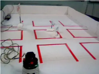
Figure 1: Experimental setup

Figure 2: Environment setup for Robot Motion Planning

WIRELESS CAMERA RADIO AV RECEIVER

TV TUNER

WIRELESS CAMERA

AUDIO OUTPUT

VIDEO & AUDIO INPUT TO THE USB CABLE

KHEPERA POWER CABLE

RS232 CABLE

[image:4.595.217.378.427.547.2]

(5)

[image:5.595.139.450.66.468.2]

Figure 3: Snapshot taken at different stages of motion planning

(a) Robot moves from initial position to the first junction

(b) After detecting the road sign the robot moves towards the next junction in right direction

(c) After detecting the road sign the robot moves towards the next junction in left direction

(d) After detecting the road sign the robot moves towards the next junction in left direction towards the goal

(e) Robot reaches the goal position and stop

5. CONCLUSION

This paper proposed road map based path planning by Khepera robot having perception of a predefined road map. The road map path based planning is introduced here using the image matching techniques. In this paper, weconsidered a new concept for matching images. Hausdorff distance to measure the degree of the similarity between two images, and used Chaos to optimize the search process of Hopfield Neural Network, derived a new energy formulation for Hopfield Neural Network based image matching method, where the problem of image matching is treated with the minimization of an energy function by estimating. The proposed method is free from size and rotational variance and requires insignificantly small time for the matching process. Through extensive experiments the effectiveness of the proposed technique is verified. The work may be realized in the

automatic control of the vehicle in autopilot mode in a predefined road map.

6. REFERENCES

[1] K. Fleischer and H.–H. Nagel: Machine–Vision–Based Detection and Tracking of Stationary infrastructural Objects beside Innercity Roads. In: Proc. of the IEEE Intelligent Transportation Systems Conf. (ITSC), August 25–29, 2001, Oakland, CA, USA, pp. 525–530.

(6)

[3] Bijita Biswas, Amit Konar, Achintya K. Mukherjee “Image matching with fuzzy moment descriptors”, Engineering Applications of Artificial Intelligence 14 (2001) 43-49

[4] Biswas, B., Konar, A., Mukherjee, A.K., 1996. Fuzzy moments for digital image matching. Proceedings of the International Conference on Control, Automation, Robotics and Computer Vision (ICARCV '96), Singapore

[5] Biswas, B., Mukherjee, A.K., Konar, A., 1995. Matching of digital images using fuzzy logic. AMSE Publication 35 (2), 7-11.

[6] Y. He, H. Wang, and B. Zhang, “Color-based road detection in urban traffic scenes,” IEEE Trans. Intell. Transport. Syst., vol. 5, no. 4, pp.309– 318, 2004 [7] L. C. Gomez and O. Fuentes, “Color-Based Road Sign

Detection and Tracking”, Proceedings Image Analysis and Recognition (ICIAR), Montreal, CA, August 2007. [8] D. Song, H.-L. Lee, J. Yi, and A. Levandowski,

“Vision-based motion planning for an autonomous motorcycle on ill-structured roads,” Autonomous Robots, vol. 23, no. 3, pp. 197–212, 2007.

[9] Shi, Z., Huang, S., Feng, Y.: Artificial Neural Network Image Matching. Microelectronics and Computer, 20

(2003) 18-21

[10] Nasrabadi, N.M., Li, W.: Object Recognition by a Hopfield Neural Network. IEEE Trans.Systems, Man, and, Cybernetics, 21 (1991) 1523-1535

[11] Li, W., Lee, T.: Hopfield Neural Networks for Affine Invariant Matching. IEEE Transactions on Neural Networks, 12 (2001) 1400-1410

[12] Huttenlocher, D.P., Kalanderman, G.A.: Comparing Image Using the Hausdorff distance. IEEE Trans. Pat. Anal. Machine Intel, 15 (1993) 850-863

[13] Chen, L., Aihara, K.: Chaotic Simulated Annealing by a Neural Network Nodal with Transient Chaos. Neural Networks, 8 (1995) 915-930