Comparisons and Contrasts between Asymmetry and Nestedness in Interacting Ecological Networks

http://dx.doi.org/10.4236/oje.2014.411055

How to cite this paper: Corso, G. and Britton, N.F. (2014) Comparisons and Contrasts between Asymmetry and Nestedness in Interacting Ecological Networks. Open Journal of Ecology, 4, 653-661. http://dx.doi.org/10.4236/oje.2014.411055

Comparisons and Contrasts between

Asymmetry and Nestedness in

Interacting Ecological

Networks

Gilberto Corso

1*

, N. F. Britton

2

1_{Departamento de Biof sica e Farmacologia, Centro de Biociências, Universidade Federal do Rio Grande do}

Norte, Natal-RN, Brazil

2_{Department of Mathematical Sciences and Centre for Mathematical Biology, University of Bath, Bath, UK}

Email: *[email protected]

Received 1 June 2014; revised 3 July 2014; accepted 15 July 2014

Copyright © 2014 by authors and Scientific Research Publishing Inc.

This work is licensed under the Creative Commons Attribution International License (CC BY).

http://creativecommons.org/licenses/by/4.0/

Abstract

We compare and contrast asymmetry and nestedness, two concepts used in the characterisation of the specialist-generalist balance in bipartite ecological interaction networks. Our analysis is rele-vant to mutualistic networks such as those consisting of flowering plants and pollinators, or fruit-ing plants and frugivores, or antagonistic networks such as those consistfruit-ing of plants and herbi-vores, in an ecological community. We shall refer to the two sets of species in the bipartite net-work as plants and animals, the usual but not the only ecological situation. By asymmetry we mean either connectivity asymmetry or dependence asymmetry, which are essentially equivalent. Asymmetry expresses two attributes: generalists interact preferentially with specialists, and spe-cialists avoid interacting with each other. Nested patterns, in principle, should express these same two features and one more: the presence of a core of interactions among generalists. We compute

the full set of perfectly nested patterns that are possible in an L × L matrix with N interactions,

representing an ecological network of L plants and L animals, and point out that the number of

nested arrangements grows exponentially with N. In addition, we analyse asymmetry for the full

set of perfectly nested patterns, and identify extremes of asymmetry inside the universe of nested patterns. The minimal asymmetry is marked by a modular core of interactions between species that are neither specialists nor generalists. On the other hand, the case of maximal asymmetry is formed by a set of few generalists and many specialists with equal connectivity. The stereotypic case of nestedness with a core of interactions among generalists has intermediate asymmetry.

*

Keywords

Bipartite Interaction Networks, Nestedness, Asymmetry, Ecology of Communities

1. Introduction

The contemporary way to look at an ecological community is through the lens of an interaction network; in this approach the pattern formed by the interactions is more important than the particular species that take part in the tangled interplay of the interactions. Despite the widespread acceptance for employing networks as good theo-retical models to investigate ecological communities, their characterisation remains a delicate matter. Many tools from network theory and statistics have been used in this enterprise [1]-[4], but not all are based on a clear mathematical background, and this leads to possible ambiguity.

A scientific theory should employ intelligible concepts to produce clear statements, otherwise any attempt at falsification will be ineffective or dubious. We state this methodological remark because the aim of this paper is to clarify concepts. We shall focus on two concepts that are used, and sometimes interchanged, to understand the specialist-generalist balance in bipartite interaction networks (BINs): asymmetry and nestedness.

The ecological idea behind connectivity asymmetry is that generalist species are typically connected to spe-cialists. Such a pattern may contribute to stability [5]-[7]. In an abstract way, we can formulate connectivity asymmetry as the following principle: species tend to interact with species with the maximum possible differ-ence in their number of interactions. Specialists tend to interact with generalists, and neither generalists nor spe-cialists tend to interact with each other. We shall see later that connectivity asymmetry is essentially equivalent to dependence asymmetry, where species prefer to interact with species with the maximum possible difference in their dependences on each other. Asymmetry indices may be defined for qualitative networks, where informa-tion is only available on whether or not plant species i interacts with animal species j, or for quantitative net-works, where in addition the strength of the interaction is quantified. In the literature, dependence asymmetry was explored initially for qualitative networks by Vásquez and Aizen [8], and then for quantitative networks by Bascompte and co-authors [9] and, using an entropy-based approach, by Blüthgen and co-authors [10].

Nestedness was first introduced to describe patterns of species composition on islands [11], then adapted to describe patterns that commonly occur in plant-pollinator BINs by [12], and had been used widely to describe many BINs. A nested BIN contains, at the same time, three different aspects [13]: 1) a core of generalists that interact with other generalists; 2) many generalists that interact with specialists; and 3) an absence of interac-tions between specialists. Nestedness indices are normally only defined for qualitative networks. Although there is no consensus in the literature about the best way to define an index to quantify nestedness [11], most authors agree that a gap-free matrix is perfectly nested [14] [15]. It means that, once we place rows and columns in de-creasing order of their sums, the final matrix representation of a perfectly nested BIN should contain no empty site with an occupied site to its right or below it.

In this methodological manuscript we proceed by comparison, exploring similarities and contrasts between asymmetry and nestedness. Since nestedness indices for BINs are based on qualitative data, the comparison re-quires us to use qualitative data for measures of asymmetry as well. We start by introducing connectivity asym-metry for qualitative networks and stating its main properties, and show that it is equivalent to dependence asymmetry. After that we take a matrix of given size and occupancy, and give an asymptotic expression for the number of possible perfectly nested arrangements. We then calculate the connectivity asymmetry for all per-fectly nested arrangements, focusing on the nested patterns of maximal and minimal asymmetry. In the conclu-sion, we discuss the results in the context of the literature of BINs, and explore the possibility of employing connectivity asymmetry as a tool in the analysis of qualitative BINs.

2. Theoretical Analysis

1 if plant species and animal species interact, 0 if not.

ij

i j

a = 

 (1)

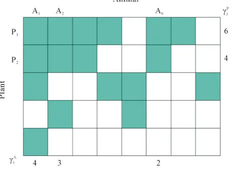
This is the object that represents the qualitative information in the BIN. An illustrative example of the bipar-tite networks is given in Figure 1. It has dimensions L_P×L_A, where L_P and L_A are the numbers of plant and animal species in the community. We can project the information in the matrix onto connectivity vectors of plants, P

( )

P

i

k = k , and animals, A

( )

A j

k = k , by

1 1

and .

A P

L L

P A

i ij j ij

j i

k a k a

= =

=

∑

=

∑

(2)

The quantity k_iP gives the number of animal species that interact with plant species i, and k_jA the number of plant species that interact with animal species j. Finally we define N, the total number of interactions in the network or the total number of occupied sites in the matrix, by

1 1 1 1

,

P A A P

L L L L

P A

i j ij

i j j i

N k k a

= = = =

=

∑

=

∑

=

∑∑

(3)

and the density ρ of occupied sites by

ρ

=N

(

L LA P

)

.

2.1. Connectivity Asymmetry for Qualitative BINs

Let us define the L_P×L_A connectivity asymmetry matrix C=

( )

c_ij between plant i and animal j by

(

)

if plant species and animal species interact,

0 if not.

P A P A

i j i j

ij

k k k k i j

c

 _{− +}

 = 

 (4)

(An alternative definition, cij = kiP−kjA max

(

kiP,kAj

)

, gives similar results but is less mathematically tractable. Others [16] have omitted the modulus signs in defining similar quantities, but we are only interested in the ab-solute value of the difference between the connectivities of plant species i and animal species j.) Note that

[image:3.595.200.432.457.627.2]

0≤cij<1, and cij=0 in the symmetric case where the plant and the animal have equal connectivity, while maximal asymmetry is achieved when maximally specialist plants

(

kiP =1

)

interact with maximally generalist

Figure 1.An illustration of a typical adjacency matrix. The shaded boxes indicate interaction between plant and animal species. We highlighted row and columns of plant P2 and

animal A6. The dependence of these species is 2 4

P

k = and

6 2

A

k = . The asymmetry between these particular plant and

animal species is _2,6 4 2 1 4 2 3

c = − =

animals

(

kA_j =L_P

)

, or maximally specialist animals

(

k_jA=1

)

interact with maximally generalist plants

(

P

)

i A

k =L . In these cases cij=

(

LP−1

) (

LP+1

)

or cij =

(

LA−1

) (

LA+1

)

, which tend to 1 as LP → ∞ or A

L → ∞ respectively.

The global connectivity asymmetry c of a BIN is given by averaging c_ij over all the occupied sites of the matrix,

, 1 1

1 1

.

A P

L L

ij ij

i j j i

c c c

N N = =

=

∑

=

∑∑

(5)

Note that, despite a claim to the contrary for a similar index [16], this is not well approximated by

(

)

P A P A

L −L L +L . In particular, L_P−L_A

(

L_P+L_A

)

is zero if L_P =L_A, and we shall see later that c does not share this property.

It is interesting to note that, by definition, c is a quantity that depends only on the total number of interac-tions of species, k_iP for plants i and kA_j for animals j. The number of interactions, in its turn, is not affected by permutations of lines or columns in the matrix. In this way c does not require any matrix-packing proce-dure that is commonly used in the estimation of nestedness [11].

2.2. Dependence and Connectivity Asymmetry

The dependence ∆_ijP of a plant species i on an animal species j is a measure of how much plant species i de-pends on animal species j, and is defined for a qualitative network by

1 if plant species and animal species interact,

0 if not.

P P

P i i

ij

k i j

δ

 =

 ∆ = 

 (6)

The L_P×L_A dependence matrix ∆P _{for plants is defined by} P

( )

P ij

∆ = ∆ . In this way, a maximally special-ist plant species i that interacts with just one animal species j has a maximal dependence ∆ =Pij

δ

iP =1 on that

species, while a maximally generalist plant species i that interacts with all L_A animal species has minimal de-pendence ∆ =Pij

δ

iP=1LA for every animal species j, with 0

P i

δ

→ as L_A→ ∞. Similarly, the dependence A

ij

∆ of an animal species j on a plant species i is defined by

1 if animal species and plant species interact,

0 if not.

A A

j j

A ij

k j i

δ

 =

 ∆ = 

 (7)

and the L_P×L_A dependence matrix _∆A _{for animals is defined by} A

( )

A ij

∆ = ∆ . (Note that we retain the con-vention of using the rows of a matrix for plants and the columns for animals, so that the second index in ∆_ijA refers to the dependent species.) Just as for plants, a maximally specialist animal species has dependence 1 on the single plant species that it interacts with, while a maximally generalist animal species has dependence 1LP on each and every plant species.

The dependence asymmetry d_ij between animal species i and plant j is a quantity that express the difference between the two dependences, and is given by

(

)

if plant species and animal species interact,

0 if not.

P A P A

i j i j

ij

i j

d δ δ δ δ

 − +

 = 

 (8)

The L_P×L_A dependence asymmetry matrix is given by D=

( )

d_ij . (Just as for connectivity asymmetry, the alternative definition d_ij = δ_iP −δA_j max

(

δ δ_iP, _jA

)

gives similar results but is less mathematically tractable. This alternative definition is essentially that of [9], but adapted to a qualitative network.) Note that 0≤d_ij<1. Moreover, C=D, since c_ij =d_ij =0 if plant species i does not interact with animal species j, while if there is an interaction,

1 1

.

1 1

P A P A A P

i j i j j i

ij P A P A A P ij

i j i j j i

k k

c d

k k

δ δ δ δ

δ δ δ δ

− − −

= = = =

+ + + (9)

2.3. The Number of Nested Patterns

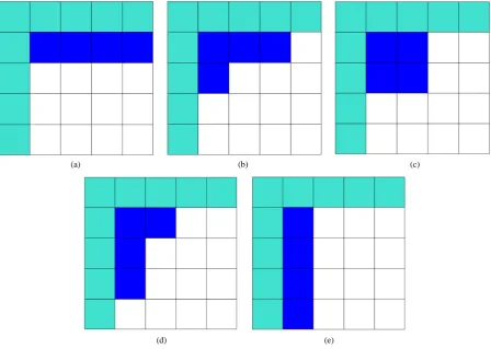
The number of nested patterns can be estimated analytically or algorithmically. For sake of simplicity we restrict our analysis to the case of a square matrix of size L L× . In the first step of the construction of an artificial nested pattern we have to be sure that all species have at least one link. To fulfil this statement we set in the ma-trix an outer shell of occupied elements; this procedure may be visualised in the set of Figure 2. In this set the empty sites are white and the occupied sets are grey—the clear grey sites are the outer shell. The number of elements in the outer shell, N_shell, is given by 2L−1.

Recall that N is the total number of occupied sites in the matrix, and define N_int to be the number of ele-ments of the matrix that do not belong to the external shell; in this way N=N_shell+N_int. In Figure 2 the inter-nal elements are shown in a dark grey tone. To compute the total number of different perfectly nested patterns,

χ, we start with the simplest case where N_int≤ −L 1. To illustrate this case we show in Figure 2 five matrices with LP=LA=5 and Nint=4; the nested matrices of this set of figures correspond to all possible

arrange-ments of matrices with N_int =4 and no gaps in their arrangement. Indeed, the arrangement of inner elements follows a partition of a positive integer, in this case, the partition of 4. In number theory, a partition of a positive integer N counts the total number of ways that N may be written as a sum of positive integers. The number of partitions of N is given by the partition function p N

( )

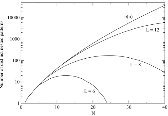
[17].

In Figure 3 we show χ versus the number of occupied sites N. The main function depicted in the graphic is the partition function p N

( )

. In the case that N_int≤ −L 1 the number of distinct nested patterns is equal to

( )

p N itself. For N_int> −L 1, the number of distinct nested patterns is smaller than p N

( )

because partitions of N that extend beyond the length of the square (vertically or horizontally) are not allowed. A generic expres-sion of the χ is given by p_L−_1,L−₁

(

N_int

)

, the number of partitions of Nint into a sum of no more than L−1

in-tegers with no term greater than L−1 in the sum. The curve of χ is symmetric relative to N_max =

(

L−1

)

2 2;

(a) (b) (c)

[image:5.595.90.539.367.686.2]

(d) (e)

[image:6.595.179.451.81.269.2]

Figure 3. A curve of the total number of different perfectly nested pat-terns, χ, for several cases. The partition function p (N) is the upper boun-dary curve of χ. We illustrate the cases of L = 6, 8 and 12; for these cases the χ depart from the curve because a finite lattice cannot effect all the in-teger partitions.

indeed, for N>N_max, χ becomes the same as another related quantity, the number of different anti-nested patterns, or nested patterns formed by empty sites instead of occupied ones.

An asymptotic expression for p N

( )

in the limit as N→ ∞ is given [18] by

( )

1

expπ 2 3,

4 3

p N N

N

 (10)

and the modified partition function p_L−_1,L−₁

( )

N has similar asymptotic behaviour. In this equation the

expo-nential term dominates the expression for large N. The conclusion we take from this expression is that for a large number of interactions, N, the number of possible nested arrangements grows exponentially. Such a property seems not to encourage the use of nestedness to produce characteristic indices of BINs, and we discuss this point in the conclusion.

2.4. Asymmetry Distribution among Nested Patterns

To understand how connectivity or dependence asymmetry and nestedness are related we plot histograms of c

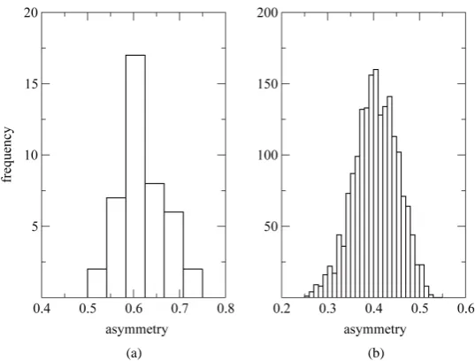
for all the multiplicity of nested patterns. This procedure enables us to grasp the differences in c that are in-side the set of possible nested arrangements for a given L and N. Figure 4 shows, for L = 11, two distinct cases: in (a) the occupation is low, N_int=10, and in (b) it is high, N_int=30. As

ρ

=

(

N_shell+N_int

)

L2 we have

0.26

ρ= in (a) and ρ=0.42 in (b). Although the two pictures show similar distribution patterns, we high-light two differences between them. The first is that values of asymmetry are larger for smaller ρ, because ge-neralists in this case are connected largely to specialists, producing sites of high asymmetry. On the other hand, for high ρ the matrix is densely occupied and specialists become scarce, decreasing the average asymmetry of the sites. The second point to which we call attention is that χ is much larger for high ρ, a result that comes directly from Figure 3 or, in a similar way, from Equation (10).

We now stress the cases of patterns of maximal and minimal c among the set of all different nested patterns. The point here is to understand the configurations that produce the extremes of c in the histograms of Figure 4. This question is important because we can understand the appearance of matrices of high and low asymmetry. In Figure 5 we show, for a square matrix with L=11 and N_int=16, the matrices of lowest c in (a) and of highest c in (c). The case (c) is not unique, since a reflected figure along the diagonal of the square has the same asymmetry. The case of minimal c is easy to understand: all elements of the internal square have

, 0

i j

[image:7.595.179.448.82.286.2]

(a) (b)

Figure 4. Two histograms illustrating the distributions of asymmetry, where L = 11 and the number of occupied sites is (a) low, Nint = 10, and

(b) high, Nint = 30.

(a) (b) (c)

Figure 5. The complete nested matrices illustrating to three cases of dependence asymmetry for a same ρ: in (a) the mi-nimal c, in (b) the average c and in (c) the maximal c. We use in this simulation L=11 and N_int=16. The case of minimal c is characterised by a solid modular structure while the maximal c is formed by two additional generalists. The typical case of a nested pattern is depicted in (b), the average c among the ensemble of nested patterns.

maximum number of specialists; the consequence of this choice is the complete exclusion of species that are neither maximally generalists nor specialists. We plot also in Figure 5(b) the median of histogram. This pattern resembles a typical nested pattern, and we stress this point in the discussion.

3. Discussion and Final Remarks

[image:7.595.91.540.332.491.2]

It is interesting to note that the pictorial examples of nested patterns shown in scientific articles [12] [19] show an intermediate c between these two extreme cases.

We recall three aspects of a nested pattern that we have outlined in the introduction: a) a core of generalists that interact with another generalist; b) many generalists that interact with specialists; and c) an absence of inte-ractions between specialists. A generalist connected to many specialists gives origin to sites of high asymmetry, and an interaction of a specialist with another specialist produces sites of zero asymmetry; the absence of this pattern in nested networks also increases the asymmetry. In this way, cases (b) and (c) are typical of networks with high asymmetry. On the one hand, a core of generalists interacting with generalists leads to sites of low asymmetry, which contribute to decreasing the asymmetry. This picture agrees with the last sentence of the pre-vious paragraph: the stereotype of an optimal nested pattern is something “in between” two extremes of asym-metry dependence. We remark that the ensemble of perfectly nested patterns does not necessarily fulfill condi-tions (a) and (b). Indeed, inside the spectrum of perfectly nested patterns, the case of minimal c does not fulfil condition (b) and the case of maximal c does not follow condition (a). However, the nested patterns around the peak of distribution of c follows conditions (a), (b) and (c), in agreement with the ecological concept of nestedness [12] [13] [19].

In this work we call attention to one aspect that has not been stressed in the literature [11] [19]. The nested patterns have an internal multiplicity of states; and furthermore, the number of perfectly nested patterns grows exponentially with the number of occupied sites, Equation (10). However, despite the fact that perfectly nested

patterns are asympotically like ek N, the total number of patterns is asympotically like ekN. In this way the number of perfectly nested structures is a very small fraction of the total number of patterns. This justifies, in a statistical way, the use of nested patterns for the construction of indices. In addition, the use of a nestedness in-dex usually occurs in comparison with an ensemble of random matrices that have the same distribution of P

i

k

and kA_j [7] [11] [20]. Such a procedure, known as the R3 null model, restricts strongly the number of nested structures with a given N and enables a reasonable use of a nestedness index. For the case of perfectly nested pattern there is just one pattern for fixed P

i

k and k_jA, but for a generic case this point is unclear. We note that there is an analytic result in the literature that can be used to clarify this point. In the work [21] there is a proof that the nestedness index

ν

depends only on P

i

k and kA_j to be calculated; however, there is not yet a well established relation of

ν

with other nestedness indices like the NODF [22] or the Temperature of Atmar [23].

Connectivity or dependence asymmetry seems to be a good candidate to characterise qualitative BINs, and we give at least two reasons for that. It is easy to compute because it is not necessary to perform a matrix-packing procedure, besides we compute c by counting c_{i j,} over matrix elements, which can be done in one line of a program in R. The second point is that asymmetry has a direct ecological interpretation: it computes the imbal-ance of species connectivities in the network. On the other side, the difficulty of using c as an index is that it should be properly normalised or exhaustively compared with null models [11] [24]. Without a comprehensive test of c against matrix sizes and occupancy, it is not expected that c could be used to compare matrices of different L and ρ. At this moment we are working on a well normalised asymmetry index that we intend to use to distinguish antagonist from mutualist networks.

Acknowledgements

Financial support to Gilberto Corso from CNPq (Conselho Nacional de Desenvolvimento Científico e Tec-nológico) is acknowledged.

References

[1] Bascompte, J. and Jordano, P. (2013)Mutualistic Networks, Princeton University Press, Princeton.

[2] Fointaine, C. (2013) Abundant Equals Nested. Nature, 500, 411-412. http://dx.doi.org/10.1038/500411a

[3] Dormann, C.F., Fründ, J., Blüthgen, N. and Gruber, B. (2009) Indices, Graphs and Null Models:Analyzing Bipartite Ecological Networks. The Open Journal of Ecology, 2, 7-24. http://dx.doi.org/10.2174/1874213000902010007

[4] Ings, T.C., Montoya, J.M., Bascompte, J., Blüthgen, N., Brown, L., Dormann, C.F., et al. (2009) Ecological Net-works—Beyond Food Webs. Journal of Animal Ecology, 78, 253-269.

http://dx.doi.org/10.1111/j.1365-2656.2008.01460.x

[6] Suweis, S., Simini, F., Banavar, J.R. and Maritan, A. (2013) Emergence of Structural and Dynamics Properties of Ecological Mutualistic Networks. Nature, 500, 449-452. http://dx.doi.org/10.1038/nature12438

[7] Thébault, E. and Fontaine, C. (2010) Stability of Ecological Communities and the Architecture of Mutualistic and Trophic Networks. Science, 329, 853-856. http://dx.doi.org/10.1126/science.1188321

[8] Vázquez, D.P. and Aizen, M.A. (2004) Asymmetric Specialisation: A Pervasive Feature of Plant-Pollinator Interac-tions. Ecology, 85, 1251-1257. http://dx.doi.org/10.1890/03-3112

[9] Bascompte, J., Jordano, P. and Olesen, J.M. (2006) Asymmetric Coevolutionary Networks Facilitate Biodiversity Maintenance. Science, 312, 431-433. http://dx.doi.org/10.1126/science.1123412

[10] Blüthgen, N., Menzel, F. and Blüthgen, N. (2006)Measuring Specialization in Species Interaction Networks. BMC Ecology, 6, 9. http://dx.doi.org/10.1186/1472-6785-6-9

[11] Ulrich, W., Almeida-Neto, M. and Gotelli, N.J. (2009) A Consumer’s Guide to Nestedness Analysis. Oikos, 118, 3-17. http://dx.doi.org/10.1111/j.1600-0706.2008.17053.x

[12] Bascompte, J., Jordano, P, Melián, C.J. and Olesen, J.M. (2003) The Nested Assembly of Plant-Animal Mutualistic Networks. Proceedings of the National Academy of Sciences of the United States of America, 100, 9383-9387. http://dx.doi.org/10.1073/pnas.1633576100

[13] Guimarães Jr., P.R., Rico-Gray, V., dos Reis, S.F. and Thompson, J.N. (2006) Asymmetries in Specialization in Ant- Plant Mutualistic Networks. Proceedings of the Royal Society B: Biological Sciences, 273, 2041-2047.

[14] Araujo, A.I.L., Corso, G., Almeida, A.M. and Lewinsohn, T.M. (2010) An Analytic Approach to Nestedness Index of Bipartite Networks. Physica A: Statistical Mechanics and Its Applications, 389, 1405-1411.

http://dx.doi.org/10.1016/j.physa.2009.11.030

[15] Brualdi, R.A. and Sanderson, J.G. (1999) Nested Species Subsets, Gaps, and Discrepancy. Oecologia, 119, 256-264. http://dx.doi.org/10.1007/s004420050784

[16] Blüthgen, N. (2010)Why Network Analysis Is Often Disconnected from Community Ecology: A Critique and An Eco- logist’s Guide. Basic and Applied Ecology, 11, 185-195. http://dx.doi.org/10.1016/j.baae.2010.01.001

[17] Hardy, G.H. and Wright, E.M. (1938) An Introduction to the Theory of Numbers. Oxford University Press, Oxford.

[18] Hardy, G.H. and Ramanujan, S. (1918) Asymptotic Formulae in Combinatory Analysis. Proceedings of the London Mathematical Society, 17, 75-115. http://dx.doi.org/10.1112/plms/s2-17.1.75

[19] Lewinsohn, T.M., Prado, P.I., Jordano, P., Bascompte, J. and Olesen, J.M. (2006) Structure in Plant-Animal Interaction Assemblages. Oikos, 113, 174. http://dx.doi.org/10.1111/j.0030-1299.2006.14583.x

[20] Fortuna, M.A., Stouffer, D.B., Olesen, J.M., Jordano, P., Mouillot, D., Krasnov, B.R., et al. (2010) Nestedness versus Modularity in Ecological Networks: Two Sides of the Same Coin? Journal of Animal Ecology, 79, 811-817.

[21] Corso, G., Araujo, A.I.L. and Almeida, A.M. (2011) Connectivity and Nestedness in Bipartite Networks from Com-munity Ecology. Journal of Physics: Conference Series, 285, Article ID: 012009.

[22] Almeida-Neto, M., Guimarães, P.R. and Lewinsohn, T.M. (2007)On Nestedness Analyses: Rethinking Matrix Tem-perature and Anti-Nestedness. Oikos, 116, 716-722. http://dx.doi.org/10.1111/j.0030-1299.2007.15803.x