Munich Personal RePEc Archive
Modelling Time Series Count Data: An
Autoregressive Conditional Poisson
Model
Heinen, Andreas
Center of Operations research and Econometrics
July 2003
Modelling Time Series Count Data: An Autoregressive
Conditional Poisson Model
∗Andr´eas Heinen†
First Draft: November 2000 This version: July 2003
JEL Classification codes: C25, C53, G1.
Keywords: Forecast, volatility, transactions data.
Abstract
This paper introduces and evaluates new models for time series count data. The Autoregressive Conditional Poisson model (ACP) makes it possible to deal with issues of discreteness, overdispersion (variance greater than the mean) and serial correlation. A fully parametric approach is taken and a marginal distribution for the counts is spec-ified, where conditional on past observations the mean is autoregressive. This enables to attain improved inference on coefficients of exogenous regressors relative to static Poisson regression, which is the main concern of the existing literature, while mod-elling the serial correlation in a flexible way. A variety of models, based on the double Poisson distribution of Efron (1986) is introduced, which in a first step introduce an additional dispersion parameter and in a second step make this dispersion parameter time-varying. All models are estimated using maximum likelihood which makes the usual tests available. In this framework autocorrelation can be tested with a straight-forward likelihood ratio test, whose simplicity is in sharp contrast with test procedures in the latent variable time series count model of Zeger (1988). The models are applied to the time series of monthly polio cases in the U.S between 1970 and 1983 as well as to the daily number of price change durations of .75$ on the IBM stock. A .75$ price-change duration is defined as the time it takes the stock price to move by at least .75$. The variable of interest is the daily number of such durations, which is a measure of intradaily volatility, since the more volatile the stock price is within a day, the larger the counts will be. The ACP models provide good density forecasts of this measure of volatility.
∗The author acknowledges financial support from the Swiss National Science Foundation. This paper has benefited greatly from many conversations with Rob Engle. I also wish to thank Luc Bauwens, Bruce Lehmann, Richard Carson, David Veredas and seminar participants at CORE, CERGE-EI, University of Alicante, University of Exeter, University of Rotterdam, Technical University of Lisbon and participants at the Econometric Society Meeting in Venice, August 2002. The usual disclaimer applies.
1
Introduction
Many interesting empirical questions can be addressed by modelling a time series of count data. Examples can be found in a great variety of contexts. In the area of accident prevention, Johansson (1996) used time series counts to assess the effect of lowered speed limits on the number of road casualties. In epidemiology, time series counts arise naturally in the study of the incidence of a disease. A prominent example is the time series of monthly cases of polio in the U.S. which has been studied extensively by Zeger (1988) and
Br¨ann¨as and Johansson (1994). In the area of finance, besides the applications mentioned
in Cameron and Trivedi (1996), counts arise in market microstructure as soon as one starts looking at tick-by-tick data. The price process for a stock can be viewed as a sum of discrete price changes. The daily number of these price changes constitutes a time series of counts whose properties are of interest.
Most of these applications involve relatively rare events which makes the use of the normal distribution questionable. Thus, modelling this type of series requires one to deal explicitly with the discreteness of the data as well as its time series properties. Neglect-ing either of these two characteristics would lead to potentially serious misspecification. A typical issue with time series data is autocorrelation and a common feature of count data is overdispersion (the variance is larger than the mean). Both of these problems are addressed simultaneously by using an autoregressive conditional Poisson model (ACP). In the simplest model counts have a Poisson distribution and their mean, conditional on past observations, is autoregressive. Whereas, conditional on past observations, the model is equidispersed (the variance is equal to the mean), it is unconditionally overdispersed. A fully parametric approach and choose to model the conditional distribution explicitly and make specific assumptions about the nature of the autocorrelation in the series. A simi-lar modelling strategy has been explored independently by Rydberg and Shephard (1998), Rydberg and Shephard (1999b), and Rydberg and Shephard (1999a). Two generalisations of their framework are introduced in this paper. The first consists of replacing the Pois-son by the double PoisPois-son distribution of Efron (1986), which allows for either under- or overdispersion in the marginal distribution. In this context, two common variance functions will be explored. Finally, an extended version of the model is proposed, which allows for separate models of mean and of variance. It is shown that this model performs well in a financial application and that it delivers very good density forecasts, which are tested by using the techniques proposed by Diebold, Gunther, and Tay (1998).
The main advantages of this model are that it is flexible, parsimomious and easy to estimate using maximum likelihood. Results are easy to interpret and standard hypothesis tests are available. In addition, given that the autocorrelation and the density are modeled explicitly, the model is well suited for both point and density forecasts, which can be of interest in many applications. Finally, due to its similarity with the autoregressive conditional heteroskedasticity (ARCH) model of Engle (1982), the ACP model can be extended to most of the models in the ARCH class; for a review see Bollerslev, Engle, and Nelson (1994).
2
A review of models for count data in time series
Many different approaches have been proposed to model time series count data. Good reviews can be found both in Cameron and Trivedi (1998), Chapter 7 and in MacDonald and Zucchini (1997), Chapter 1. Markov chains are one way of dealing with count data in time series. The method consists of defining transition probabilities between all the possible values that the dependent variable can take and determining, in the same way as in usual time series analysis, the appropriate order for the series. This method is only reasonable, though, when there are very few possible values that the observations can take. A prominent area of application for Markov chains is binary data. As soon as the number of values that the dependent variable takes gets too large, these models lose tractability.
Discrete Autoregressive Moving Average (DARMA) models are models for time series count data with properties similar to those of ARMA processes found in traditional time series analysis. They are probabilistic mixtures of discrete i.i.d. random variables with suitably chosen marginal distribution. One of the problems associated with these models seems to be the difficulty of estimating them. An application to the study of daily precipi-tation can be found in Chang, Kavvas, and Delleur (1984). The daily level of precipiprecipi-tation is transformed into a discrete variable based on its magnitude. The method of moments is used to estimate the parameters of the model by fitting the theoretical autocorrelation function of each model to its sample counterpart. Estimation of the model seems quite cumbersome and the model is only applied to a time series which can take at most three values.
McKenzie (1985) surveys various models based on ”binomial thinning”. In those
mod-els, the dependent variableytis assumed to be equal to the sum of an error term with some
prespecified distribution and the result of yt−1 draws from a Bernoulli which takes value
1 with some probability ρ and 0 otherwise. This guarantees that the dependent variable
takes only integer values. The parameter ρ in that model is analogous to the coefficient
on the lagged value in an AR(1) model. This model, called INAR(1), has the same au-tocorrelations as the AR(1) model of traditional time series analysis, which makes it its discrete counterpart. This family of models has been generalised to include integer valued ARMA processes a well as to incorporate exogenous regressors. The problem with this type of models is the difficulty in estimating them. Many models have been proposed and the emphasis was put more on their stochastic properties than on how to estimate them.
Hidden Markov chains, advocated by MacDonald and Zucchini (1997) are an extension of the basic Markov chains models, in which various regimes characterising the possible values of the mean are identified. It is then assumed that the transition from one to another of these regimes is governed by a Markov chain. One of the problems of this approach is that it there is no accepted way of determining the appropriate order for the Markov chain. Whereas in some cases there is a natural interpretation for what might constitute a suitable regime, in most applications, and in particular in the applications considered in this paper, this is not the case. Another problem is that the number of parameters to be estimated can get big, especially when the number of regimes is large. Finally, the results are, in most cases, not very easy to interpret.
Harvey and Fernandes (1989) use state-space models with conjugate prior distributions. Counts are modeled as a Poisson distribution whose mean itself is drawn from a gamma
distribution. The Gamma distribution depends on two parameters a and b which are
treated as latent variables and whose law of motion isat|t−1 =ωat−1 and bt|t−1 = ωbt−1.
filter is used to update the latent variables.
In the static case overdispersion is usually viewed as the result of unobserved hetero-geneity. One way of dealing with this problem is to keep an equidispersed distribution, but introduce new regressors in the mean equation which are believed to capture this het-erogeneity. Zeger and Qaqish (1988) apply ths intuition to the time series case and add lagged values of the dependent variable to the set of regressors in a static Poisson regression. They adopt a generalised linear model formulation in which conditional mean and variance are modeled instead of marginal moments. For count data, the authors propose using the
Poisson distribution with thelog, its associated link function. The mean is set equal to a
linear combination of exogenous regressors and the time series dependence is accounted for by a weighted sum of past deviations of the dependent variable from the linear predictor:
log(µt) = x
′
tβ+
Pq
i=1θi
h
log(yt∗−i)−x′t−iβi where y∗t = max(yt−i, c). These models have
not been used very much in applications. One of the weaknesses of this specification is that had hoc assumptions are needed to handle zeros.
Zeger (1988) extends the generalised linear models and introduces a latent multiplicative
autoregressive termǫt with unit expectation , varianceσ2 and autocorrelationρǫ(τ) which
is responsible for introducing both autocorrelation and overdispersion into the model. The
dependent variable is assumed to be a function of exogenous regressorsxt with conditional
mean µt = exp(xtβ), where β is the coefficient of interest. Conditionally on the latent
variable, the model is equidispersed (E[yt|ǫt] =V[yt|ǫt] =µtǫt), but the marginal variance
depends both on the marginal mean and its square: E[yt] =µt and V[yt] = µt+σ2µ2t. In
order to estimate this model with maximum likelihood, one would need to specify a density
foryt|ǫt and for ǫt. In most cases, no closed-form solution would be available. Instead, a
quasilikelihood method is adopted, which only requires knowledge of mean, variance and
autocovariances of yt. Given estimates of the parameters of the latent variable, obtained
by the method of moments, the variance-covariance matrixV of the dependent variable is
formed: V =A+σ2ARǫA, whereA=diag(µi) andR is the autocorrelation matrix of the
latent variable Rj,kǫ =ρǫ(|j−k|). The quasilikelihood approach then consists in using the
inverse of the variance matrix V as a weight in the first order conditions. Since inversion
ofV is quite cumbersome when the time series is long, an approximation is proposed. This
method can be viewed as a count data analog of the Cochrane-Orcutt method for normally distributed time series in which all the serial correlation is assumed to come from the error term. The method has been applied to sudden infant death syndrome by Campbell (1994). While conceptually this method is quite close to what is proposed in this paper, there are nonetheless important differences in that it is fundamentally a static model with a correction for autocorrelation in the same sense as Generalised Least Squares (GLS) are, whereas the model in this paper is an explicitly dynamic one. The interest is not limited to getting correct inference about the parameters on the exogenous variables but also lies in adequately capturing the dynamics of the system. In order to achieve this, a more parametric approach is taken, which, among other things, allows forecasting.
3
The ACP Model
Poisson case.
LetFtdenote the information available on the series up to and including timet. In the
simplest model, the counts are generated by a Poisson distribution
Nt|Ft−1∼P(yt, µt), (3.1)
with an autoregressive conditional intensity as in the ACD model of Engle and Russell (1998) or the conditional variance in the GARCH (Generalised Autoregressive Conditional Heteroskedasticity) model of Bollerslev (1986):
E[Nt|Ft−1] =µt=ω+ p
X
j=1
αjNt−j+ q
X
j=1
βjµt−j , (3.2)
for positiveαj’s,βj’s andω.
We call this model the Autoregressive Conditional Poisson (ACP hereafter). The following properties of the unconditional moments of the ACP can be established.
Proposition 3.1 (Unconditional mean of the ACP(p,q)). Provided thatPmax(p,q)
j=0 (αj+
βj)<1, the ACP(p,q) is stationary and its unconditional mean is
E[Nt] =µ=
ω
1−Pmax(p,q)
j=0 (αj+βj)
.
This proposition shows that, as long as the sum of the autoregressive coefficients is less than 1, the model is stationary and the expression for its mean is identical to the mean of an ARMA process. In the sequel we will focus attention on the models based on the ARMA(1,1) structure, because, as in the GARCH and the ACD literature, these are the most commonly used ones. The mean equation is then given as:
E[Nt|Ft−1] =µt=ω+α1Nt−1+β1µt−1 . (3.3)
Proposition 3.2 (Unconditional variance of the ACP(1,1) Model). The uncondi-tional variance of the ACP(1,1) model, when the condiuncondi-tional mean is given by (3.3) is equal to
V[Nt] =σ2 =
µ(1−(α1+β1)2+α21)
1−(α1+β1)2 ≥µ .
Proof of Proposition 3.2. Proof in appendix
Proposition 3.2 shows that unconditionally the ACP exhibits overdispersion, even though it uses an equidispersed conditional distribution. The model is overdispersed, as long as
α1 6= 0 and the amount of overdispersion is an increasing function ofα1 and also, to a lesser
extent, of β1. The following proposition establishes an expression for the autocorrelation
function of the ACP.
Proposition 3.3 (Autocorrelation of the ACP(1,1) Model). The unconditional au-tocorrelation of the ACP(1,1) model is given by
Corr[Nt, Nt−s] = (α1+β1)s−1
α1(1−β1(α1+β1))
1−(α1+β1)2+α2
1
.
This holds also for all models with mean equation given by 3.3, such that µt
Nt =
α2 1 1−(α1+β1)2+α21
Proof of Proposition 3.3. Proof in appendix
The result in Proposition 3.3 holds also for all the models developed in the following sections (DACP1, DACP2, GDACP, GDACP1 and GDACP2) and for both the exponential and the Weibull versions of the ACD model of Engle and Russell (1998) with an ARMA(1,1) structure. The score (shown in Appendix 2, section 9.1) can easily be seen to be equal to zero in expectation, and this is true even if (3.1) does not hold. This means that the Poisson assumption provides a quasilikelihood estimator. In other terms, even if we misspecify the distribution, the estimates of the parameters of he conditional mean will still be consistent. It is of interest in this model to test whether there is significant autocorrelation. This
corresponds to testing the joint hypothesis that α1 = β1 = 0 in the ACP(1,1) model.
In most time series applications a massive rejection can be expected. This can be done very simply with a likelihood ratio test (LR). The statistic will be equal to twice the difference between the unrestricted and the restricted likelihoods, which follows the usual
χ2 distribution with two degrees of freedom. Both the restricted and the unrestricted
models are easy to estimate. The simplicity of this test contrast sharply with the difficulties associated with tests and estimation of the autocorrelation of a latent variable in the model of Zeger (1988) which have been recently addressed in Davis, Dunsmuir, and Wang (2000).
4
The DACP Model
This section introduces two models based on the double Poisson distribution, which differ only by their variance function. The DACP1 has its variance proportional to the the mean, whereas the DACP2 has a quadratic variance function.
In some cases one might want to break the link between overdispersion and serial corre-lation. It is quite probable that the overdispersion in the data is not attributable solely to the autocorrelation, but also to other factors, for instance unobserved heterogeneity. It is also possible that the amount of overdispersion in the data is less than the overdispersion resulting from the autocorrelation, in which case an underdispersed marginal distribution might be appropriate. In order to account for these possibilities the Poisson is replaced by the double Poisson, introduced by Efron (1986) in the regression context, which is a natural extension of the Poisson model and allows one to break the equality between conditional mean and variance. This density is obtained as an multiplicative mixture with parameter
γ of the Poisson density of the observation y with mean µ and of the Poisson with mean
equal to the observationy, which can be thought of as the likelihood function taken at its
maximum value. If we denoteP(y, µ) = e−yµ!µy, we can write the double Poisson as:
f(y|µ, γ) =γ12P(y, µ)γP(µ, µ)1−γ
After simplification the expression for the Double Poisson density is:
f(y|µ, γ) =³γ12e−γµ
´µe−yyy
y!
¶ µ
eµ y
¶γy
, (4.1)
forµ >0 and γ >0.
f(y|µ, γ) is not strictly speaking a density, since the probabilities don’t add up to 1, but
Efron (1986) shows that the value of the multiplicative constant c(µ, γ), which makes it
into a proper density is very close to 1 and varies little across values of µ and γ. He also
1
c(µ, γ) = 1 +
1−γ
12µγ
µ
1 + 1
µγ
¶
.
As a consequence, he suggests maximising the approximate likelihood (leaving out the highly nonlinear multiplicative constant) in order to estimate the parameters and using the correction factor when making probability statements using the density.
The advantages of using this distribution are that it can be both under- and
overdis-persed, depending on whether γ is smaller or larger than 1. This will prove particularly
useful in a later section of this paper, when two separate processes are used for the variance and mean, because this density ensures that there is no possibility that the conditional mean become larger than the conditional variance, which would not be allowable with strictly overdispersed distributions. In the case of the Double Poisson (DP hereafter), the distributional assumption (3.1) is replaced by the following:
Nt|Ft−1∼DP(µt, γ). (4.2)
It is shown in Efron (1986) (Fact 2) that the mean of the Double Poisson is µt and that
the variance is approximately equal to µt
γ. Efron (1986) shows that this approximation is
highly accurate, and it will be used in the more general specifications.
For the simplest model, called the DACP1, the variance is a multiple of the mean:
V[Nt|Ft−1] =σt2=
µt
γ . (4.3)
The coefficientγ of the conditional mean will be a parameter of interest, as values different
from 1 will represent departures from the Poisson distribution. The following proposition gives an expression for the variance of the DACP1.
Proposition 4.1 (Unconditional variance of the DACP1(1,1) Model). The uncon-ditional variance of the DACP1(1,1) model, when the conuncon-ditional mean is given by 3.3 is equal to
V[Nt] =σ2=
1
γ
µ(1−(α1+β1)2+α21)
1−(α1+β1)2 ≥
µ ,
if γ ≤1.
Proof of Proposition 4.1. Proof in appendix
Proposition 4.1 shows that, like the ACP, the DACP1 model exhibits overdispersion,
when-everγ ≤1. In empirical work, the most frequently observed case is when the overdispersion
generated by the autocorrelation is insufficient to match the unconditional overdispersion
in the data, and thereforeγ <1. It is however conceivable that we findγ ≥1, which would
mean that the parameter in the unconditional distribution compensates for the overdisper-sion due to the autocorrelation. The advantage of the Double Poisson over other count distributions is precisely that such cases can be accounted for. Results for the ACP(1,1)
are obtained by settingγ = 1. The amount of overdispersion is an increasing function ofα1
and also, to a lesser extent, ofβ1. When α1 is zero, the overdispersion of the model comes
exclusively from the Double Poisson distribution and is purely a function of the parameter
γ, a measure of the departure from the Poisson distribution. The overdispersion can be
σ2 µ =
1
γ
1−(α1+β1)2+α21
1−(α1+β1)2
.
Another popular way of parameterising the dispersion is to allow for a quadratic relation between variance and mean, and this, along with the distributional assumption (4.2) defines the DACP2:
V[Nt|Ft−1] =σt2 =µt+δµ2t . (4.4)
This parameterisation can be used along with the expression for the variance of the double
Poisson, replacingγin (4.1) with µt
σt =
1
1+δµt. One potential problem with this specification,
however, is that even though it can accommodate some underdispersion whenδ <0, it is
then not possible to exclude negative values of the variance whenµt<−1δ. For this reason,
when it is expected that the conditional distribution will be underdispersed, the DACP1 should be preferred. The variance of the DACP2 takes a somewhat different form from the one of the DACP1, which is the object of the following proposition.
Proposition 4.2 (Unconditional variance of the DACP2(1,1) Model). The uncon-ditional variance of the DACP2(1,1) model, when the conuncon-ditional mean is given by 3.3 is equal to
V[Nt] =σ2 =
µ(1−(α1+β1)2+α21)(1 +δµ)
1−δα21−(α1+β1)2 ≥
µ ,
whenever δ≥0.
Proof of Proposition 4.2. Proof in appendix
This shows that the DACP2 is overdispersed in general (when δ > 0, which is the case
considered in this paper) and that overdispersion is an increasing function of the parameters of the mean equation and of the dispersion parameter. The two effects cannot be separated here as they could in the case of the DACP1. As mentioned earlier on, the autocorrelation of both versions of the DACP is identical to the one of the ACP, which means that the dispersion properties of the marginal density do not affect the time series properties of the model. It can be seen from the Hessian of the DACP1, (shown in Appendix 2, section 9.2), that the cross derivative has an expectation of zero, so the expected Hessian is a
block-diagonal matrix. This means that it is efficient to estimate γ independently from θ and
that the variance of the estimators of the mean and dispersion are just the inverse of the diagonal elements of the Hessian. This is no longer the case for the DACP2, as can be seen from its likelihood in section 9.2.
In both DACP specifications excess overdispersion can be tested with a simple Wald test
forγ = 1 in the DACP1 and for δ= 0 in the DACP2. Autocorrelation can be tested with
a likelihood ratio test of a model in which the autoregressive parameters of the conditional mean are restricted to be zero against a more general alternative. One potential problem may lie in the fact that the double Poisson models are estimated by approximate maximum likelihood. The test is really an approximate likelihood ratio where the approximation error
log³c(µu,γu)
c(µr,γr) ´
is assumed to be close to zero.
formulations, however, the mean and variance are bound to covary in a rather restricted way. In the DACP1, by construction, the mean and variance have a correlation of 1. In the DACP2 this isn’t the case, but mean and variance have to move together. Whenever the mean increases, the variance increases as well. This means that the models proposed so far are, by virtue of their distributional assumption, not only autoregressive models for the mean, but also autoregressive heteroskedasticity models. However the form of their heteroskedasticity might be too restrictive in certain situations, for example in the case of a rare disease, one does not really know whether a disease is spreading out or whether the large number of cases was just an isolated occurrence. When the number of cases is small it tends to be followed by small counts and both mean and variance are then small. On the contrary, a larger count can be followed either by a large count (the disease is spreading out) or by a small count, in which case the mean does not change much, but the variance increases significantly as a result of this uncertainty. In order to deal with series of that sort, more flexible models have to be considered.
5
Extension to time-varying variance
This section introduces two different types of generalisations of the double Poisson models. The first, which will be called Generalised DACP (GDACP), adds a GARCH variance function to the DACP. The second type of extension consists of modelling the dispersion parameters of the DACP1 and DACP2 as autoregressive variables and the resulting models are called the Generalised DACP1 (GDACP1) and Generalised DACP2 (GDACP2).
The advantage of the Double Poisson distribution is that it allows for separate models of the mean and of the dispersion. In the regression applications of Efron (1986), the mean is made to depend on one set of regressors and the dispersion depends on a different set, via a logistic link function. This is a natural parameterisation for the cases most often analysed in the biostatistics literature, where certain variables are thought to affect the dispersion of the dependent variable. For example, in the toxoplasmosis data analysed by Efron (1986), which involves a double logistic, the dependent variable is the percentage of people affected by the disease in every city, the annual rainfall in every city is the explanatory variable and the sample size in each city determines the amount of overdispersion. However, in the time series case, which is the focus of this paper, there are in general no such variables. This is obviously true for univariate time series but it is also the case for many other applications. In the univariate time series context dispersion will be modelled as a function of the past of the series. Two alternative specifications will be proposed, one in terms of the variance and the other in terms of the dispersion parameter.
The model written in terms of the variance will be examined first. This is a natural way to think about this problem since in the modelling of economic time series, based implicitly on thinking about the normal distribution, the focus has been more on models of the variance than on models of the dispersion. Moreover in terms of writing an autoregressive model of dispersion, it is not obvious what the lagged variable should be. As a consequence, it will also be difficult to calculate the theoretical unconditional moments of the model. In the case of variance however, one can adopt GARCH type variance functions and choose conditional variance as the lagged variable. With a GARCH process for the conditional variance, the dispersion parameter of the double Poisson can be expressed as a function of both the conditional mean and variance. The mean specification will be the same as in (3.2), but in addition, the conditional variance will be modelled as:
ht≡E
£
From here on coefficients appearing in the conditional mean are indexed by 1 and coefficients of the conditional variance process are indexed by 2. For this specification, the dispersion
coefficientγ of the simple double Poisson is expressed in terms of the conditional mean and
variance of the process:
γt=
µt
ht
. (5.2)
The likelihood of the GDACP model is shown in Appendix 2, section 9.4. The following proposition gives an expression for the unconditional variance of the GDACP when both the conditional mean and variance have one autoregressive and one moving average parameter.
Proposition 5.1 (Unconditional variance of the GDACP(1,1,1,1) Model). The variance of the generalised model is given by:
V[Nt] =σ2=
ω2
(1−α2−β2)
(1−(α1+β1)2+α21)
(1−(α1+β1)2)
.
Proof of Proposition 5.1. Proof in appendix
The variance is a product of the unconditional mean of the variance process and a term depending on the mean equation parameters. Some insight can be gained by dividing both sides of this equation by the unconditional mean of the counts and making use of (3.2):
σ2 µ =
ω2
(1−α2−β2)
ω1(1−(α1+β1)2+α21)
(1 +α1+β1) .
It is now apparent that the overdispersion of the GDACP is a product of the long term mean
of the variance process and of a term which is decreasing in α1 and β1. This somewhat
counterintuitive result is due to the fact that the variance process gives rise to most of the overdispersion and that the autoregressive parameters of the mean, while increasing
the unconditional variance, actually increase the mean even more for a given ω1, which in
aggregate decreases the overdispersion.
It is of interest to see how the GDACP relates to the models presented in the previous
sections. The GDACP model nests the plain double Poisson (obtained when α1 = β1 =
α2 = β2 = 0) with γ = ωω21 in the case of the DACP1 and δ =
ω2−ω1
ω2 1
in the case of the
DACP2) and the plain Poisson (obtained whenα1 =β1 =α2=β2= 0 andω2 =ω1), but it
does not nest non-trivial ACP or DACP models (whereα1 6= 0 andβ1 6= 0). A consequence
of this is that it is not possible to test the GDACP against the previous models with a test of nested hypotheses. One would have to resort to tests of non-nested hypotheses, which in the present case would be quite cumbersome, due to the fact that the conditional mean and variance are unobserved autoregressive processes.
The GDACP model is convenient because it has many features which make it familiar for time series econometricians, however it does not nest simpler models like the DACP. This makes testing the general model against the more restrictive ones difficult. To remedy this, one can model the dispersion parameter of the double Poisson directly. Unlike the variance, when modelling time-varying dispersion, there is no natural candidate lagged dependent variable. As a consequence a logistic link function will be used as in Efron (1986):
γt=
M
1 + exp (−λt)
, (5.3)
λt=ω2+α2
Nt−1−µt−1
õ
tγt
+β2λt−1 .
M is the maximum possible overdispersion, which, as in Efron (1986), will not be estimated
but set by trial and error. In all the applications it will be set to 10. Unlike in the previous model, the unconditional moments are not easy to compute explicitly. We can nonetheless establish the following result:
Proposition 5.2 (Unconditional variance of the GDACP1(1,1,1,1) and GDACP1(1,1,1,1) Models). The variance of the generalised model is given by:
V[Nt] =σ2=a
(1−(α1+β1)2+α21)
(1−(α1+β1)2)
,
where a = E[µt
γt] in the case of the GDACP1 and a = E[µt+δtµ
2
t] in the case of the
GDACP2.
Proof of Proposition 5.2. Proof in appendix
In the present formulation, however, the regressor is a martingale difference sequence
which makesλta stationary ARMA process. It can be seen that this dispersion model nests
the DACP1 (whenα2 =β2 = 0 and the ACP (when in addition,ω2 =log(M−1)), but not
the DACP2. It is possible however to build a model which nests the DACP2 by setting δ
defined in (4.4) to be a function ofλas in (5.3). These models will be called GDACP1 and
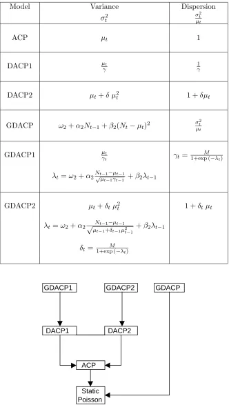
GDACP2 respectively by reference to the DACP1 and DACP2 models that they generalise. Table 1 contains a summary of the model specifications and the chart on page 24 shows how the various models relate to each other. Testing the time-varying overdispersion in the GDACP1 and GDACP2 can be done with a likelihood test against the null hypothesis of DACP1 and DACP2 respectively. Gurmu and Trivedi (1993) consider artificial regression tests for dispersion models which could easily be generalised to time-varying overdispersion. These tests would then be very similar to GARCH tests with the exception that they are based on the deviation instead of the residuals.
An advantage of the double Poisson over any of the overdispersed densities alluded to earlier becomes more obvious now. The double Poisson distribution can be either over- or underdispersed, which means that the conditional variance can be either larger or smaller than the conditional mean. With a strictly overdispersed distribution, there would be a problem 111111111each time the mean gets larger than the variance in the GDACP or when the dispersion gets smaller than 1 for the GDACP1 or GDACP2, which could happen in the numerical optimisation of the likelihood or when making out-of-sample predictions. There is no constraint on the parameters of the model which could ensure that this does not happen. With the double Poisson, however, there is no need to worry about this possibility. The models can easily be generalised to include explanatory variables. It is possible to multiply the conditional mean, variance or overdispersion by a function of exogenous regressors in exactly the same way as in Zeger (1988). In the case of the Poisson, this can be done by using the natural link function, which is the exponential. Instead of using
directly µt and ht, one could use µtexpXδ1 and htexpXδ2 as the new conditional mean
6
Data analysis
In order to demonstrate how the models work, they are applied to two datasets in completely different areas. The first is a medical example and the second is an application to stock market data.
6.1 Incidence of poliomyelitis in the U.S.
The first application of the model is to the monthly number of cases of poliomyelitis in the United States between 1970 and 1983, which was analysed as an example in Zeger (1988). Zeger estimated three models, two of which assume that repeated observations are independent and follow a negative binomial distribution in one case or have a constant coefficient of variation in the other case. The model proposed by Zeger considers that there is a latent process which generates overdispersion and autocorrelation. The time series of polio cases seems to have become a benchmark for time series count models. It has been analysed by Br¨ann¨as and Johansson (1994), who study properties of different estimators for the parameters of the latent variable in the Zeger model which are responsible for overdispersion and autoregression. Davis, Dunsmuir, and Wang (2000) propose a test for the presence of a latent variable and a correction for the standard errors of the coefficients on exogenous regressors based on asymptotic theory. They apply their method to the polio series to show that their theoretical standard errors are close to simulated ones. Jorgensen, Lundbye-Christensen, Song, and Sun (1999) propose a nonstationary state space model and apply it to the same dataset. Fahrmeir and Tutz (1994) reports results from the estimation of a log-linear Poisson model which includes lagged dependent variables.
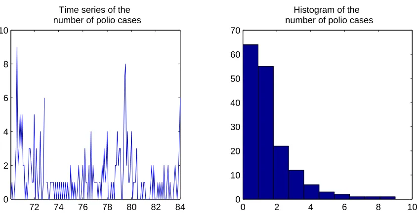
Upon examining the series of polio cases (see Figure 2), it is not at all obvious whether this dataset provides evidence of declining incidence of polio in the U.S. which is one of the questions of interest. The histogram reveals that the counts are very small with more
than 60% of zeros. The series is clearly overdispersed with a mean of 1.33 and a variance
of 3.50. Figure 3 shows the autocorrelogram of the number of polio cases after an outlier
of 14 in November 1972, which could well be a recording error, has been taken out. There is significant autocorrelation in levels and squares, and there is a clear pattern in the sign of the autocorrelation, which is first positive, then negative and positive again at very high lags.
Results from models without exogenous regressors are reported in table 2. The outlier of 14 has been taken out for the remainder of the analysis, as it had a strong impact on some of the coefficients. Models are evaluated on the basis of their log-likelihood, but also on the
basis of their Pearson residuals, which are defined as: ǫt= √T1−KNtσ−tµt, where a correction
for the number of degrees of freedom was used. If a model is well specified, the Pearson residuals will have variance one and no significant autocorrelation left. Autocorrelation is
tested with a likelihood ratio test (LR) which gives a test statistic of 57.4 much larger than
the χ2[2] 5% value of 5.99. The simplest model is the ACP which, while providing a good
fit and capturing some autocorrelation, leaves an overdispersed residual with a variance
of 1.70. The DACP1 and DACP2 correct for this, reducing this variance to 1.05 and .96
respectively. Both a Wald test, which in this case is the same as a simple t-test of the null
that γ = 0 in the DACP1 or δ = 0 in the DACP2, and a likelihood ratio (LR) test reject
the ACP model. As was to be expected, the double Poisson makes it possible to fit the autocorrelation and the overdispersion at the same time.
capturing the time series aspect of the data while missing some of the dispersion. They imply a relatively high degree of persistence with the sum of the autoregressive parameters
around .75 for most models. Amongst the more general models the GDACP2 performs
best in terms of the dispersion, since it leaves a standard residual with a variance of 1.00,
but the GDACP1 seems to provide a slightly better fit. The GDACP1 is preferred to the DACP1 that it nests as shown by a LR test statistic of 8, but it is not possible to reject the
DACP2 against the more general GDACP2 (the LR test statistic is.8). For an overview of
the models, see table?? and the chart on page 24. The model which is formulated with a
GARCH variance function does not perform as well as the dispersion models.
Figure 4 shows the autocorrelations of the Pearson residuals for the models considered so far. There is a great overall reduction in the level of autocorrelation below the Bartlett
confidence interval which lies at.154, except for very few values. The Ljung-Box statistic for
autocorrelation which does not allow to reject the null hypothesis of zero autocorrelations for any lags in the original series is reversed for all lags for the standardised residuals of the models. The pattern observed in the autocorrelogram of the series has been replaced by a pattern at a higher frequency. It can be expected that this pattern will disappear with the inclusion of seasonality dummies. Figure 5 reveals that all models have very small autocorrelations in squares and have lost the low frequency pattern that is present in the original series.
In order to compare the results to the results of Zeger (1988), models using the same set of regressors were estimated. These include trigonometric seasonality variables at yearly and half yearly frequencies as well as a time trend, since interest lies in whether or not the present dataset provides evidence of declining incidence of polio in the U.S. The results, shown in table 3 are qualitatively similar to Zeger’s results. In all the models the coefficient on the time trend is negative and insignificant. This coefficient is systematically smaller in absolute value across all the specifications than what Zeger reports. The coefficients of the seasonality variables are more or less the same as in Zeger (1988). The results seem to be even closer to what Fahrmeir and Tutz (1994) report in Table 6.2 than to Zeger’s results. Magnitudes vary a little but the signs are always the same. In all models, the seasonality variables are significant as a group. Again autocorrelation is tested and the null of no serial
correlation is rejected with a test statistic of 24 very much in excess of the 5.99 value under
the null. The overall picture for the models including exogenous regressors is the same as for the ones which do not. LR tests reject the Poisson model in favour of the double Poisson. The DACP2 is the best amongst the simpler models both in terms of the likelihood and in the modelling of dispersion, since it leaves an almost perfectly equidispersed residual. The GDACP1 fits better, but does slightly worse than the DACP2 in terms of the residuals. A LR test rejects the DACP1 in favour of the GDACP1, but it is not possible to reject the DACP2 against the alternative hypothesis of GDACP2 at the 5% level.
6.2 Daily number of price changes
The second application of the model that is to the daily number of price change durations
of.75$ on the IBM stock on the New York Stock Exchange from May 28 1997 to December
29 1998, which represents 504 obervations. A .75$ price-change duration is defined as the
time it takes the stock price to move by at least.75$. The variable of interest is the daily
number of such durations, which is a measure of intradaily volatility, since the more volatile the stock price is within a day, the more often it will cross a given threshold and the larger the counts will be. Midquotes from the Trades and Quotes (TAQ) dataset will be used to
compute the number of times a day that the price moves by at least.75$, using the ”five
second rule” of Lee and Ready (1991) to compute midquotes prevailing at the time of the trade. For robustness it is required that the following midquote not revert the price change.
Let us denote by St the midquote price of the asset and by τn the times at which the
threshold is crossed:
τn+1 = inf
t {t > τn:|St−Sτn| ≥d} (6.1)
The durations are then defined as ∆tn=τn+1−τnand the object of interest is the daily
number of such durations, which is a measure of intradaily volatility. Unlike the volatility that can be extracted from daily returns, for example with GARCH, the counts are a daily measure based on the price history within a day and this will contain information that volatility measures based on daily data are missing. For such a series interest lies amongst other things in forecasting, as volatility is an essential indicator of market behaviour as well as an input in many asset pricing problems.
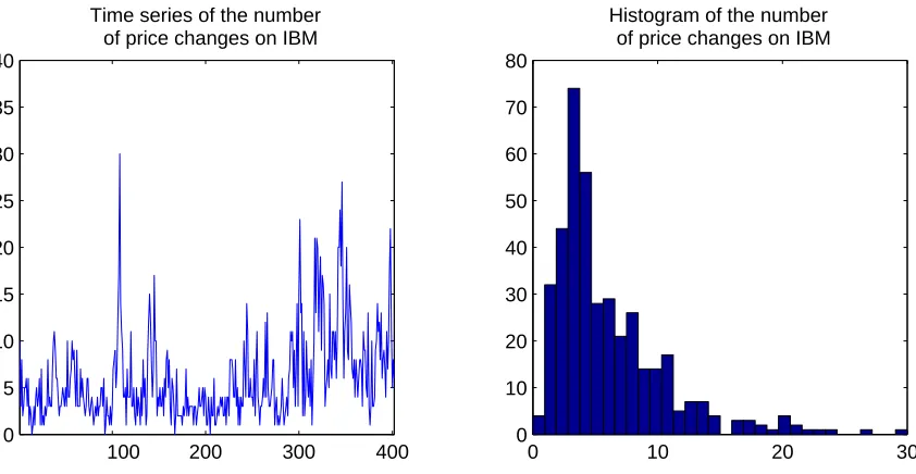
As can be seen from the plotted series in Figure 9, the counts have episodes of high and low mean as well as variance, which suggest that autoregressive modelling should be appropriate. The histogram reveals that the data range from 0 to 30. The data is
overdispersed with a mean of 5.98 and a variance of 20.4. Also, Figure 8 shows that the
autocorrelations of the series in level and squares are clearly significant up to a relatively
large number of lags (the Bartlett’s 95% confidence interval under the null of iid is .10).
Significant autocorrelation is also present in the third and fourth powers, although to a lesser degree.
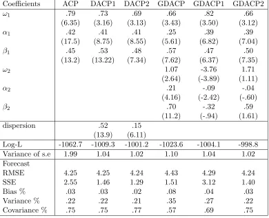
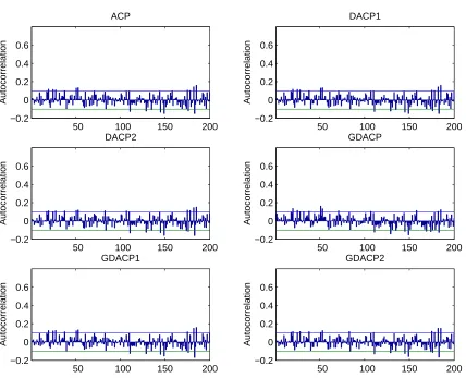
A series of models is estimated, which range from the simple ACP to the most general GDACP and the results are reported in table 4. Most parameters are significant with
t-statistics well above 2. All the models imply that the series is quite persistent withα1+β1
in the order of .82 to .94. The GDACP implies that the variance is also very persistent
with a value of.912 for the sum of the autoregressive parameters. Again the simple Poisson
show very low autocorrelation, which indicates that the models capture the serial correlation in the first four moments well.
The models are also evaluated with respect to the quality of their out-of-sample fore-casts. The models are estimated on a starting sample of 202 observations from May 28 1997 to March 16 1998, then a one-step-ahead forecast is calculated and the model is reestimated for every period from March 17 1998 to December 29 1997 with all the available informa-tion, which represents 200 one-step ahead foreasts. First the quality of the point forecasts from each one of the models is evaluated. The Root Mean Squared Errors (RMSE) of the various models are quite close to each other. The models which do best are the DACP2 and GDACP2, but the ACP and he DACP1 do almost as well. In terms of the Standardised
Sum of Errors the DACP2 performs best with a variance of 1.29, the closest to one from all
models. A decomposition of the forecasting error shows that the bias is very small in most models which means that the forecasts are right on average. The variance proportion of
the forecast for most models is around.25% which means that the variance of the forecast
and the variance of the original are quite close to each other. The remaining part of the forecasting error is unsystematic forecasting error. It is a good sign for the forecasts that most of the error is of the unsystematic type. Using that measure, the DACP2 is again seen to be the best with 77% of the forecasting error being of the unsystematic type.
Another way to test the accuracy of the models is to evaluate how good they are at forecasting the density of the counts out-of-sample. For this purpose the method developed by Diebold, Gunther, and Tay (1998) is used, which consists in computing the cumulative probability of the observed values under the forecast distribution. If the density from the model is accurate, these values will be uniformly distributed and will have no significant autocorrelation left neither in level nor when raised to integer powers. In order to assess
how close the distribution of the Z variable is to a uniform, quantile plots of Z against
quantiles of the uniform distribution are shown. The closer the plot is to a 45%-line, the closer the distribution is to a uniform. The quantile plots of the various models are shown in figure 12. The Z statistic for most models is quite close to the 45%-line. The GDACP1 is the model which performs best. The Poisson model gives too little weight to large observations as is reflected in the fact that the curve is clearly below the 45%-line
between.6 and 1. This is present to a certain degree in all of the plots, but less so for more
sophisticated models. The ACP and GDACP1 give too little weight to zeros whereas all other models attribute too much probability mass to them. All the models seem to have difficulty with the right tail: they cannot quite accommodate as many large values as are present in the data. Diebold, Gunther, and Tay (1998) propose to graphically inspect the correlogram along with the usual Bartlett confidence intervals. For the present case, this
means that all correlations smaller in absolute value than .141 can be considered not to
7
Conclusion
This paper introduces new models for time series count data. These models have proved very flexible and easy to estimate. They make it possible to correct standard errors and improve inference on parameters of exogenous regressors compared to Static Poisson regression like other methods, particularly the one proposed by Zeger (1988), which has attracted a lot of attention recently, while modelling the time series dependence in a more flexible way. It is shown that these models perform well and can explain both autocorrelation and dispersion in the data. The biggest advantage of this framework is that it is possible to apply straightforward likelihood based tests for autocorrelation or overdispersion. Finally this method also makes it possible to perform point and density forecasts, which successfully pass a series of forecast evaluation tests. An interesting question is how this model can be generalised in a multivariate framework and this is the object of future research.
8
Appendix 1
Proof of Proposition 3.1. Same as the proof of lemma 1 in Engle and Russell (1998).
Proof of Proposition 3.2. Upon substitution of the mean equation in the autoregressive intensity, one obtains:
µt−µ=α1(Nt−1−µ) +β1(µt−1−µ),
µt−µ=α1(Nt−1−µt−1) + (α1+β1)(µt−1−µ).
Squaring and taking the expectation gives:
E[(µt−µ)2] =α21E
£
(Nt−1−µt−1)2¤+ (α1+β1)2E£(µt−1−µ)2¤ .
Using the law of iterated expectations and substituting the conditional variance σt−1 for
its expression, one gets:
E£
(µt−µ)2
¤
=α21E[µt−1
γ ] + (α1+β1)
2E£
(µt−1−µ)2¤ . (8.1)
Collecting terms, one gets:
V[µt] =E[(µt−µ)2] =
α21µ γ(1−(α1+β1)2)
. (8.2)
Now, applying the following property on conditional variance
V[y] =Ex
£
Vy|x(y|x)¤
+Vx
£
Ey|x(y|x)¤
, (8.3)
to the counts, one obtains:
E£
(Nt−µ)2
¤
=E£
(Nt−µt)2
¤
+E£
(µt−µ)2
¤
. (8.4)
Again using the law of iterated expectations, substituting the conditional variance σt for
Proof of Proposition 3.3. As a consequence of the martingale property, deviations between
the timetvalue of the dependent variable and the conditional mean are independent from
the information set at timet. Therefore:
E[(Nt−µt)(µt−s−µ)] = 0 ∀s≥0.
By distributingNt−µt, one gets:
Cov[Nt, µt−s] =Cov[µt, µt−s] ∀s≥0. (8.5)
By the same ”non-anticipation” condition used above, it must be true that:
E[(Nt−µt)(Nt−s−µ)] = 0 ∀ s≥0.
Again, distributingNt−µt, one gets:
Cov[Nt, Nt−s] =Cov[µt, Nt−s] ∀ s≥0. (8.6)
Now,
Cov[µt, µt−s] =α1Cov[Nt, µt−s+1] +β1Cov[µt, µt−s]
= (α1+β1)Cov[µt, µt−s]
= (α1+β1)sV[µt].
The first line was obtained by replacingµtby its expression, the second line by making use
of 8.5, the last line follows from iterating line two.
Cov[µt, µt−s+1] =α1Cov[µt, Nt−s] +β1Cov[µt, µt−s].
Rearranging and making use of 8.6, one gets:
Cov[Nt, Nt−s] =
1
α1Cov[µt, µt−s+1]−
1
βCov[µt, µt−s]
= 1
α1(1−β(α+β)) (α1+β1)
sV[µ t].
Finally,
Corr[Nt, Nt−s] =
1
α1
(1−β1(α1+β1)) (α1+β1)s
V[µt]
V[Nt]
.
Replacing V[µt] and V[Nt] by their respective values, the result follows. It can be seen
easily that this proposition holds for all models, such that µt
Nt =
α2 1 1−(α1+β1)2+α2
1
. It can be verified that this is true not only for the ACP, but also for the DACP1, the DACP2, the GDACP, the GDACP1 and the GDACP2.
Proof of Proposition 4.1. This proof is similar to the proof of Proposition 4.1. When
sub-stituting the conditional varianceσt2 for its expression, instead of 8.1, one gets:
E£
(µt−µ)2
¤
=α21E[µt−1+δµ2t−1] + (α1+β1)2E
£
(µt−1−µ)2
¤
.
Similarly, instead of 8.2, one gets:
V[µt] =E[(µt−µ)2] =
α21µ(1 +δµ)
1−α21δ−(α1+β1)2
Now, applying 8.3 to the counts, one obtains 8.4. The result then follows after applying the same steps as in the previous proof.
Proof of Proposition 5.1. This proposition can be proved by proceeding in a similar fashion
as in the Proof of 3.2, but making use of the expression for the conditional varianceht. As
a result of the first step, instead of 8.2, one obtains:
V[µt] =E[(µt−µ)2] =
α21E[ht−1]
1−(α1+β1)2
. (8.7)
It can be seen from 5.1 that:
E[ht] =
ω2
1−α2−β2
. (8.8)
Applying property 8.3, making use of 8.8 and after simplification, one gets the announced result.
Proof of Proposition 5.2. This proposition can be proved by proceeding in a similar fashion
as in the Proof of 3.2, but making use of the expression for the conditional varianceht. As
a result of the first step, instead of 8.2, one obtains:
V[µt] =E[(µt−µ)2] =
α21a
1−(α1+β1)2 , (8.9)
where ais as defined in the Proposition. Applying property 8.3 and simplifying, one gets
the announced result.
9
Appendix 2: Likelihood functions, score, Hessian
9.1 The ACP
For the ACP, the likelihood is
lt(θ) =Ntln(µt)−µt−ln(Nt!),
whereθis a vector containing all the parameters of the autoregressive conditional intensity
and the conditional intensity µt is autoregressive as in (3.2). The score and Hessian take
the very simple form:
∂lt
∂θ =
µ
Nt−µt
µt
¶
∂µt
∂θ ,
∂2lt
∂θ2 =−
Nt
µ2t ∂µt
∂θ
µ
∂µt
∂θ
¶′
,
where
∂µt
∂θ =z
′
t+ p
X
s=1
βs
∂µt−s
∂θ , (9.1)
and
9.2 The DACP1
For the DACP1 the likelihood is:
lt(θ, γ) =
1
2ln (γ)−γµt+Nt(ln (Nt)−1)−ln (Nt!) +γNt
µ
1 + ln
µ
µt
Nt
¶¶
,
whereθis a vector containing all the parameters of the autoregressive conditional intensity
and the conditional intensityµt is autoregressive as in 3.2. Differentiating with respect to
θand γ,
∂lt
∂θ =γ
Nt−µt
µt ∂µt ∂θ ∂lt ∂γ = 1 2 1
γ + (Nt−µt) +Ntln
µ
µt
Nt
¶
.
The first condition with respect to θ is just the first order condition FOC) of the ACP
multiplied by the dispersion parameterγ. Taking the expectation, one gets:
E
·
∂lt
∂θ
¸
= 0.
The DACP1 is therefore a quasi maximum likelihood estimator: it is consistent as long as the mean is correctly specified, even if the true density is not double Poisson. The Hessian is given by:
∂2lt
∂θ∂θ′ =− γ Nt
µ2t
∂µt ∂θ µ ∂µt ∂θ ¶′
∂2lt
∂θ∂γ =
Nt−µt
µt
∂µt
∂θ ∂2lt
∂γ2 =−
1 2
1
γ2 ,
where ∂µt
∂θ and ztare as in (9.1) and (9.2).
Taking the expectation of the cross-derivative, one gets:
E
·
∂2lt
∂θ∂γ
¸
= 0.
The cross derivative has an expectation of zero, so the expected Hessian is a block-diagonal
matrix, which means that it is efficient to estimate γ independently from θ and that the
variance of the estimators of the mean and dispersion are just the inverse of the diagonal elements of the Hessian.
9.3 The DACP2
For the DACP2 the likelihood is more complicated. It can be obtained from the likelihood of the DACP1 by the following transformation:
Lt(θ, δ) = 12ln (1 +δµt)−µt(1 +δµt) +Nt(ln (Nt)−1)−ln (Nt!)
+Nt(1 +δµt)
µ
1 + ln
µ
µt
Nt
¶¶
,
whereθis a vector containing all the parameters of the autoregressive conditional intensity
and the conditional intensityµt is autoregressive as in 3.2. Differentiating with respect to
θand δ and denotingγt= 1 +δµt and xt=Nt
³
1 + ln³µt
Nt ´´ yields: ∂Lt ∂θ = 1 γt µ
−2δ +Nt
µt −
1
γt
(1 +δxt)
¶ ∂µt ∂θ ∂Lt ∂δ = 1 γt µ −µt
2 −
1
γt
(µt+xt)
¶
.
It can be seen, by settingδ equal to zero in the score with respect to the parameters of the
mean, that one gets back the first order condition of the Poisson model:
∂Lt
∂θ =
Nt−µt
µt
∂µt
∂δ .
The Hessian is:
∂2Lt
∂θ∂θ′ =
−1
γt2
µ
1
2+δ
Nt
µt
+2δ
γt
(1 +δxt)
¶ ∂µt ∂θ µ ∂µt ∂θ ¶′
∂2Lt
∂θ∂γ =
−1
γt2
µ
1
2+Nt+xt
1−δ2µ2t
γt2
¶
∂µt
∂θ ∂2Lt
∂γ2 =
µ
µt
γt
¶2µ
1
2 +
2
γt
(µt+xt)
¶
Again ∂µt
∂θ andzt are as in (9.1) and (9.2).
9.4 The GDACP
The likelihood function of the GDACP is:
lt(θ1, θ2)) =
1 2ln µ µt ht ¶ −µ 2 t ht
+Nt(ln (Nt)−1)−ln (Nt!) +
Ntµt
ht
µ
1 + ln
µ
µt
Nt
¶¶
,
whereµt and htare defined respectively in 3.2 and in 5.1, and where θ1 = [ω1, α1, β1] and
θ2 = [ω2, α2, β2].
The score of the model is given by
∂lt
∂µt
=
µ
1
2µt
+ 2Nt−µt
ht
+ Nt
ht ln µ µt Nt ¶¶ ∂µt ∂θ1 ∂lt ∂ht = µ 1
2ht −
µt
ht
Nt−µt
ht −
Ntµt
h2t ln
µ µt Nt ¶¶ ∂ht ∂θ2 .
∂l2t ∂θ1∂θ
′
1
=
µ −21µ2
t −
2
h1
+ Nt
µtht
¶
∂µt
∂θ1
µ
∂µt
∂θ1
¶′
∂l2t ∂θ1∂θ
′
2
=
µ
2µt
h2
t
−Nh2t
t
µ
2 + ln
µ
µt
Nt
¶¶¶
∂µt
∂θ1
∂ht
θ′2 ∂l2t
∂θ2∂θ2′
= µt
h4t
µ
Nt−µt
ht
+Nt
ht
ln
µ
µt
Nt
¶¶
∂ht
∂θ2
µ
∂ht
∂θ2
¶′
References
Bollerslev, Tim, 1986, Generalized autoregressive conditional heteroskedasticity,Journal of
Econometrics 52, 5–59.
, Robert F. Engle, and Daniel B. Nelson, 1994, Arch models, in Robert F. Engle,
and Daniel L. McFadden, ed.: Handbook of Econometrics, Volume 4 (Elsevier Science:
Amsterdam, North-Holland).
Br¨ann¨as, Kurt, and Per Johansson, 1994, Time series count data regression,
Communica-tions in Statistics: Theory and Methods 23, 2907–2925.
Cameron, A. Colin, and Pravin K. Trivedi, 1998,Regression Analysis of Count Data
(Cam-bridge University Press: Cam(Cam-bridge).
Cameron, Colin A., and Pravin K. Trivedi, 1996, Count data models for financial data,
in Maddala G.S., and C.R. Rao, ed.: Handbook of Statistics, Volume 14, Statistical
Methods in Finance (Elsevier Science: Amsterdam, North-Holland).
Campbell, M.J., 1994, Time series regression for counts: an investigation into the
relation-ship between sudden infant death syndrome and environmental temperature,Journal
of the Royal Statistical Society A157, 191–208.
Chang, Tiao J., M.L. Kavvas, and J.W. Delleur, 1984, Daily precipitation modeling by
discrete autoregressive moving average processes,Water Resources Research20, 565–
580.
Davis, Richard A., William Dunsmuir, and Yin Wang, 2000, On autocorrelation in a poisson
regression model,Biometrika 87, 491–505.
Diebold, Francis X., Todd A. Gunther, and Anthony S. Tay, 1998, Evaluating density
fore-casts with applications to financial risk management,International Economic Review
39, 863–883.
Efron, Bradley, 1986, Double exponential families and their use in generalized linear
regres-sion,Journal of the American Statistical Association 81, 709–721.
Engle, Robert, 1982, Autoregressive conditional heteroskedasticity with estimates of the
variance of U.K. inflation,Econometrica 50, 987–1008.
Engle, Robert F., and Jeffrey Russell, 1998, Autoregressive conditional duration: A new
model for irregularly spaced transaction data,Econometrica 66, 1127,1162.
Fahrmeir, Ludwig, and Gerhard Tutz, 1994, Multivariate Statistical Modeling Based on
Generalized Linear Models (Springer-Verlag: New York).
Gurmu, Shiferaw, and Pravin K. Trivedi, 1993, Variable augmentation specification tests
in the exponential family,Econometric Theory 9, 94–113.
Harvey, A.C., and C. Fernandes, 1989, Time series models for count or qualitative
obser-vations,Journal of Business and Economic Statistics 7, 407–417.
Johansson, Per, 1996, Speed limitation and motorway casualties: a time series count data
regression approach,Accident Analysis and Prevention 28, 73–87.
Jorgensen, Bent, Soren Lundbye-Christensen, Peter Xue-Kun Song, and Li Sun, 1999, A
state space model for multivariate longitudinal count data,Biometrika 96, 169–181.
Lee, Charles M., and Mark J. Ready, 1991, Inferring trade direction from intraday data,
MacDonald, Iain L., and Walter Zucchini, 1997, Hidden Markov and Other Models for
Discrete-valued Time Series (Chapman and Hall: London).
McKenzie, Ed., 1985, Some simple models for discrete variate time series,Water Resources
Bulletin 21, 645–650.
Rydberg, Tina H., and Neil Shephard, 1998, A modeling framework for the prices and times of trades on the nyse, To appear in Nonlinear and nonstationary signal processing edited by W.J. Fitzgerald, R.L. Smith, A.T. Walden and P.C. Young. Cambridge University Press, 2000.
, 1999a, Dynamics of trade-by-trade movements decomposition and models, Working paper, Nuffield College, Oxford.
, 1999b, Modelling trade-by-trade price movements of multiple assets using multi-variate compound poisson processes, Working paper, Nuffield College, Oxford.
Zeger, Scott L., 1988, A regression model for time series of counts,Biometrika 75, 621–629.
, and Bahjat Qaqish, 1988, Markov regression models for time series: A
Table 1: Summary of the model specifications. The mean in all specifications is given asµt=ω+α1Nt−1+β1µt−1.
Model Variance Dispersion
σ2t σt2
µt
ACP µt 1
DACP1 µt
γ
1
γ
DACP2 µt+δ µ2t 1 +δµt
GDACP ω2+α2Nt−1+β2(Nt−µt)2 σ
2
t
µt
GDACP1 µt
γt γt=
M
1+exp (−λt)
λt=ω2+α2N√tµ−t1−−1µγtt−−11 +β2λt−1
GDACP2 µt+δtµ2t 1 +δtµt
λt=ω2+α2√µNt−1−µt−1
t−1+δt−1µ2t−1
+β2λt−1
δt= 1+exp (M−λt)
GDACP1 GDACP2 GDACP
DACP1 DACP2
ACP
Static Poisson
Table 2: Maximum Likelihood Estimates of the Models for the Number of Cases of Polio in the U.S from January 1970 to December 1983.
The table presents the Maximum Likelihood Estimates of the Models for the Number of Cases of Polio in the U.S from January 1970 to December 1983. t-statistics are presented in parenthesis. The standard errors are computed as: ǫt= Ntσ−tµt.
Coefficients ACP DACP1 DACP2 GDACP GDACP1 GDACP2
ω1 .29 .28 .56 .12 .37 .34
(2.46) (1.49) (2.00) (.93) (1.72) (1.52)
α1 .23 .23 .36 .08 .28 .28
(4.83) (2.84) (3.47) (1.33) (2.49) (2.33)
β1 .55 .56 .21 .82 .44 .46
(5.02) (3.13) (.92) (5.31) (2.09) (2.12)
ω2 .20 -2.89 -3.45
(1.35) (-2.73) (-1.22)
α2 .06 -.21 .26
(1.51) (-2.66) (1.25)
β2 .84 -.09 -.12
(10.5) (-.24) (-.13)
dispersion .62 .53
(7.40) (2.36)
Log-L -261.8 -250.2 -247.8 -254.1 -246.2 -248.2
Variance of s.e 1.70 1.05 .96 1.11 1.02 1.00
72 74 76 78 80 82 84 0
2 4 6 8 10
Time series of the number of polio cases
0 2 4 6 8 10
0 10 20 30 40 50 60 70
[image:26.595.88.512.473.694.2]Histogram of the number of polio cases
Table 3: Maximum Likelihood Estimates of the Models for the Number of Cases of Polio in the U.S from January 1970 to December 1983, with time trend and seasonality
The table presents the Maximum Likelihood Estimates of the Models for the Number of Cases of Polio in the U.S from January 1970 to December 1983 with time trend and seasonality. t-statistics are presented in parenthesis. The standard errors are computed as: ǫt= Ntσ−tµt.
Coefficients ACP DACP1 DACP2 GDACP GDACP1 GDACP2 Zeger
ω1 .15 .37 .14 .15 .19 .15
(1.64) (1.25) (1.01) (1.29) (1.18) (1.07)
α1 .16 .23 .17 .12 .17 .18
(2.92) (2.18) (1.75) (1.78) (1.77) (1.62)
β1 .73 .52 .72 .74 .70 .71
(7.65) (2.14) (4.81) (5.01) (4.37) (4.68)
ω2 1.45 -2.72 -3.81
(1.99) (-2.18) (-1.20)
α2 .30 -.21 .33
(-2.01) (-2.48) (1.30)
β2 .51 -.07 -.13
(2.90) (-.14) (-.14)
trend -.0013 -.0021 -.0010 -.0003 -.0019 -.0014 -.0044
(-1.05) (-1.22) (-.50) (-.13) (-.57) (-.96) (-1.62)
cos12 -.26 -.24 -.29 -.02 -.18 -.25 -.11
(-3.14) (-1.89) (-2.39) (-.12) (-1.51) (-2.02) (-.69)
sin12 -.37 -.33 -.36 -.20 -.40 -.40 -.48
(-3.60) (-2.19) (-2.65) (-1.29) (-2.55) (-2.82) (-2.82)
cos6 .18 .14 .21 .02 .21 .22 .20
(1.93) (1.03) (1.45) (.14) (1.55) (1.52) (1.43)
sin6 -.40 -.41 -.38 -.20 -.40 -.40 -.41
(-4.08) (2.91) (-2.68) (-1.27) (-1.96) (-2.37) (-2.93)
dispersion .69 .38
(7.16) (2.07)
Log-L -246.5 -239.6 -238.2 -250.5 -235.9 -236.4
Table 4: Maximum Likelihood Estimates of the models for the number of price changes greater than .75$ on IBM from May 28 1997 to December 29 1998. The table presents the Maximum Likelihood Estimates of the models for the number of price changes greater than.75$ on IBM from May 28 1997 to December 29 1998, for a total of 402 observations. t-statistics are presented in parenthesis. The standard errors are computed as: ǫt= Ntσ−tµt. The initial estimation for the
forecasting exercise is performed on a sample of 202 observations from May 28 1997 to March 26 1998. The Root Mean Squared Error (RMSE) is defined aspP
(Nt−µˆt)2, the Standardised Sum of Errors (SSE) is
the out-of-sample version of the variance of the standard residuals used in-sample, and should be close to 1 if the model performs well. The forecasting error is decomposed into a bias term, a variance term and an unsystematic error term, labelled covariance term. The better the forecast, the greater the covariance term.
Coefficients ACP DACP1 DACP2 GDACP GDACP1 GDACP2
ω1 .79 .73 .69 .66 .82 .66
(6.35) (3.16) (3.13) (3.43) (3.50) (3.12)
α1 .42 .41 .41 .25 .39 .39
(17.5) (8.75) (8.55) (5.61) (6.82) (7.04)
β1 .45 .53 .48 .57 .47 .50
(13.2) (13.22) (7.34) (7.62) (6.37) (7.35)
ω2 1.07 -3.76 1.71
(2.64) (-3.89) (1.11)
α2 .21 -.09 -.04
(4.16) (-2.42) (-.60)
β2 .70 -.32 .59
(11.2) (-.94) (1.61)
dispersion .52 .15
(13.9) (6.11)
Log-L -1062.7 -1009.3 -1001.2 -1023.6 -1004.1 -998.8
Variance of s.e 1.99 1.04 1.02 1.10 1.04 1.02
Forecast
RMSE 4.25 4.25 4.24 4.43 4.29 4.24
SSE 2.55 1.46 1.29 1.51 3.12 1.40
Bias % .03 .03 .02 .08 .04 .03
Variance % .22 .22 .21 .35 .27 .22
1 2 3 4 5 6 7 8 −0.2
−0.1 0 0.1 0.2 0.3
Number of polio cases
Autocorrelation
lag (in years)
1 2 3 4 5 6 7 8
−0.2 −0.1 0 0.1 0.2 0.3
Squared number of polio cases
Autocorrelation
[image:29.595.88.510.80.290.2]lag (in years)
Figure 3: Autocorrelations of the number of polio cases. The scale for the lags is in years, which corresponds to 12 monthly observations.
1 2 3 4 5 6 7 8
−0.2 −0.1 0 0.1 0.2
ACP
Autocorrelation
1 2 3 4 5 6 7 8
−0.2 −0.1 0 0.1 0.2
DACP1
Autocorrelation
1 2 3 4 5 6 7 8
−0.2 −0.1 0 0.1 0.2
DACP2
Autocorrelation
1 2 3 4 5 6 7 8
−0.2 −0.1 0 0.1 0.2
GDACP
Autocorrelation
1 2 3 4 5 6 7 8
−0.2 −0.1 0 0.1 0.2
GDACP1
Autocorrelation
1 2 3 4 5 6 7 8
−0.2 −0.1 0 0.1 0.2
GDACP2
Autocorrelation
[image:29.595.83.514.353.698.2]1 2 3 4 5 6 7 8 −0.2
−0.1 0 0.1 0.2
ACP
Autocorrelation
1 2 3 4 5 6 7 8
−0.2 −0.1 0 0.1 0.2
DACP1
Autocorrelation
1 2 3 4 5 6 7 8
−0.2 −0.1 0 0.1 0.2
DACP2
Autocorrelation
1 2 3 4 5 6 7 8
−0.2 −0.1 0 0.1 0.2
GDACP
Autocorrelation
1 2 3 4 5 6 7 8
−0.2 −0.1 0 0.1 0.2
GDACP1
Autocorrelation
1 2 3 4 5 6 7 8
−0.2 −0.1 0 0.1 0.2
GDACP2
[image:30.595.84.508.220.561.2]Autocorrelation