Double Partitioned Ranked Set Sampling: An Efficient Estimation Technique

5

X

October 2017

Double Partitioned Ranked Set Sampling: An

Efficient Estimation Technique

K.B.Panda1, M. Samantaray2

1,2

Department of Statistics, Utkal University, Bhubaneswar, Odisha, India

Abstract: Following Ranked Set Sampling (RSS) due to McIntyre (1952), Takahasi and Wakimoto (1968), Dell and Clutter (1972) and the Median Ranked Set Sampling (MRSS) method by Muttlak(1997), a new sampling strategy has been proposed. While the newly proposed sampling design is called Double Partitioned Ranked Set Sampling(DPRSS), the estimator based thereon, besides being unbiased for the population mean, is found to be more efficient than the corresponding estimators in simple random sampling, ranked set sampling and median ranked set sampling. The theoretical findings have been supported by suitable numerical illustration.

Keywords: Simple Random Sampling, Ranked Set Sampling, Median Ranked Set Sampling, Double Ranked Set Sampling, Double Partitioned Ranked Set Sampling.

I. INTRODUCTION

McIntyre (1952) introduced a technique of sampling called Ranked Set Sampling (RSS) for estimating the mean of a finite population. This is possible where the sampling units in a survey can be more easily ranked than quantified. The estimator thus obtained comes out to be unbiased for population mean with a variance less than that of usual sample mean based on Simple Random Sampling of the same size. Muttalak (1997) proposed an estimator using Median Ranked Set Sampling(MRSS) with a view to increasing efficiency of the estimator and reducing errors in ranking. Muttalak(2003) proposed Quartile Ranked Set Sampling (QRSS) for estimating population mean is also applicable for reducing error as compared to RSS. Al-Saleh and Al-Kadiri (2000) suggested Double Ranked Set Sampling (DRSS) for estimating the population mean. According to them the ranking at second stage is easier than first stage.

II. SAMPLING METHODS

A. Ranked Set Sampling (RSS)

RSS procedure involves selection of m random samples with m units in each sample. The m units in each sample are ranked with respect to a variable of interest without actually measuring them. Then the smallest rank is measured from the first sample, the second smallest rank from second sample and the procedure is continued till the unit with highest rank is measured from themthsample.

Theorder of observations from the lowest to the highest in the m samples can be presented as x(11) x(12) ... x(1m)

x(21) x(22) ... x(2m)

x(m1) x(m2) ... x(mm)

The observations x(11),x(22) ,... x(mm) are then accurately measured to form RSS data. If m is small, then the cycle may be

repeated for r times so as to obtain a combinedsampleofsizemr.

B. Median Ranked Set Sampling (MRSS)

MRSS procedure involves selection of m random samples each of size m units from population and ranked them within each sample. If sample size m is odd, then select lowest ranks from each of the first (m-1)/2samples, the median from (m+1)/2th sample and the highest ranks from each of the last (m-1)/2 sample. If sample size m is even, then select lowest rank from each ofthe first m/2 samples and highest rank from each of the lastm/2 samples. If m is small, then the cycle may be repeated for r times to have a combined sample of sizemr. The ranked units are then quantified.

C. Partitioned Ranked Set Sampling (PRSS)

(m+1/2) set.If sample size is even, then select (p(m + 1))th rank from first (m/2) sets and (q(m+1))th rank from last (m/2) sets, where 0≤ p ≤1 and q = (1- p) then p+q=1.If m is small, then the cycle may be repeated for r times to have a combined sample of size mr.

D. Double Ranked Set Sampling (DRSS)

According to DRSS, select m3 elements from a population and divide these units randomly into m2sets eachof size m units.Apply the RSS procedure on each set to obtain m ranked set samples each of size m. Then repeat the RSS procedure again on m ranked set sample to have DRSS of size m. Then repeat the cycle for r times as per requirement.Motivated by the above works, we have proposed a new RSS technique, called Double Partitioned Ranked Set Sampling(DPRSS)along with an unbiased estimator for the population mean.The estimator thus proposed fares better than its competing estimators based on SRS, RSS and MRSS. It may be pointed out here that the proposed sampling technique can be viewed as a generalisation of Double Quartile Ranked Set Sampling (DQRSS).

E. Double Partitioned Ranked Set Sampling (DPRSS)

DPRSS technique comprises the following steps:

1) Select m3 elements from the target population and divide these elements randomly into m2 sets each of size m.

2) If sample size m is even,select the (p(m + 1))th rank from each set out of first m2/2 samples and from the second m2/2 samples the (q (m + 1))th rank from each set is selected.

3) If sample size m is odd, select from the first (m(m-1)/2) samples, the (p( m + 1))th rank from each set, the median from next m samples, and from last (m(m-1)/2) samples, select (q (m + 1))th rank from each set.

4) Here, p & q stand for pth and qthpartitioned observations, such that p + q = 1, for example p = 25% and q = 75% of the observations given. This can be done after arranging the series either inascending or in descending order visually.

5) Applying PRSS procedure on m sets obtained in above step, gives us DPRSS procedure sample of size m.

6) The whole cycle may be repeated r times to obtain a sample size of mr from DPRSS.

7) From above we have to examine mr samples out of m3r population size using DPRSS.

Here, we have to remember that, the ranking should be done by visual inspection or by any economical procedure and actual quantification is done at final stage.

To understand the above procedure, let us consider the following two example.

F. Example-1(when sample size is odd)

For odd sample size, we have to apply DPRSSO method which may be described as follows.

Let m=5, then we have to select random sample of 25 sets, each should contain 5 units. Let X(n)j(i;m) be the ith value (i=1,2,...,5) out

of the jthset (1,2,...25) at the nthstage.

After ranking, the units within each subset may be taken as    

        



011;5 01 2;5 015;5



0

1

X

,

X

...

....X

X



_,

   

       



021;5 (0)2 2;5 02 5;5



0

2

X

,

X

...

....X

X



_,

   

       



0251;5 (0)25 2;5 0255;5



0

25

X

,

X

...

....X

X



Now applying PRSSO method on each 25 sets, The first partitioned value p(m+1)th ( for p=25%) = 25% (5+1)th= 1.5th observation, which indicates the first or lowest observation, i.e., we have to assume p(m+1)thrank from each of first m(m-)/2=10sets.Similarly, the last partitioned value q(m+1)th (for q=75%)= 75%(5+1)th=4.5th observation indicates the fifth observation or largest rank from each of last 10 sets and median of each 5 sets containing 5 units will give middle 5 observations for next stage.

Using the above procedure, we arrive at

 

 



 0



1 1

5 ; 1

1

min

X

X



,

 

 



 0



10 1

5 ; 1 0

1

min

X

X



 

 



 0



11 1 5 ; M 1

1

median

X

X



,

 

 



 0



12 1 5 ; M 2

1

median

X

X



, .

.

 

 



 0



15 1 5 ; M 5

1

median

X

X



,

 

 



 0



16 1 5 ; 5 6

1

max

X

X



,

 

 



 0



17 1 5 ; 5 7

1

max

X

X



,

..and _ 1 _



₂₅ 0



5 ; 5

25

max

X

X



The above observations t can be reorganised in the following 5 sets

             



1



5 ; 1 5 1 5 ; 1 2 1 5 ; 1 1 1

1

X

,

X

...,

X

X



,              



1



5 ; 1 10 1 5 ; 1 7 1 5 ; 1 6 1

2

X

,

X

...,

X

X



,              



1



5 ; M 15 1 5 ; M 12 1 5 ; M 11 1

3

X

,

X

...,

X

X



,              



1



5 ; 5 20 1 5 ; 5 17 1 5 ; 5 16 1

4

X

,

X

...,

X

X



,              



1



5 ; 5 25 1 5 ; 5 22 1 5 ; 5 21 1

5

X

,

X

...X

X



Now, applying the same procedure once again to the above data, we get DPRSSO technique which will have p(m+1) th rank from (m-1)/2= 2 sets and choose q(m+1)th = highest rank from last 2 set and the median from middle set. Then DPRSSO partitioned sample is

 

 



 1



1 2

5 ; 1

1

min

X

X



,

 

 



 1



2 2

5 ; 1

2

min

X

X



,

 

 



 1



3 2

5 ; M

3

median

X

X



,

 

 



 1



4 2

5 ; 5

4

max

X

X



and

 

 



 1



5 2

5 ; 5

5

max

X

X



The sample observations thus obtained constitute a random sample, i.e., the observations are the realisation of 5 i.i.d. random variables. These 5 observation are to be measured.

Let m=6, Hence we have to select 63=216 units in 36 sets, each have 6 units. Let us assume that, X(n)j(i;m) be the ith

observation(i=1,2,....,6) out of the jthset (j=1,2,...36) at the nthstage. After arranging, the units within each sets, we have

             



0



6 ; 6 1 0 6 ; 2 1 0 6 ; 1 1 0

1

X

,

X

...X

X



,              



0



6 ; 6 2 0 6 ; 2 2 0 6 ; 1 2 0

2

X

,

X

...X

X



,              



0



6 ; 6 36 0 6 ; 2 36 0 6 ; 1 36 0

36

X

,

X

...X

X



The first partitioned values (p(m+1))thobservation,i.e., the lowest rank from each offirst m2/2=18 sets. The last partitioned value q(m+1)thrank,i.e,largest rank from each of last m2/2=18 observations.

Using the above procedure, we have

 

 



 0



1 1

5 ; 1

1

min

X

X



,

 

 



 0



2 1

5 ; 1

2

min

X

X



, .

 

 



 0



18 1

6 ; 1

18

min

X

X



,

 

 



 0



19 1

6 ; 6

19

max

X

X



,

 

 



 0



20 1

6 ; 6

20

max

X

X



,

and _  _



36 0



1

6 ; 6

36

max

X

X



The obtained values can be rearranged in the following 5 sets

 

 

 

 

 

 

 



1



6 ; 1 6 1

6 ; 1 2 1

6 ; 1 1 1

1

X

,

X

...X

X



,

 

 

 

 

 

 

 



1



6 ; 1 12 1

6 ; 1 8 1

6 ; 1 7 1

2

X

,

X

...X

X



,

 

 

 

 

 

 

 



1



6 ; 1 18 1

6 ; 1 14 1

6 ; 1 13 1

3

X

,

X

...X

X



,

 

 

 

 

 

 

 



1



6 ; 6 24 1

6 ; 6 20 1

6 ; 6 19 1

4

X

,

X

...X

X



,

 

 

 

 

 

 

 



1



6 ; 6 30 1

6 ; 6 26 1

6 ; 6 25 1

5

X

,

X

...X

X



,

 

 

 

 

 

 

 



1



6 ; 6 36 1

6 ; 6 32 1

6 ; 6 31 1

6

X

,

X

...X

X



Now , applying the same procedure once again to the above data, we have p(m+1)th,i.e., smallest rank out of first m/2= 3 sets and q(m+1)th, i.e., highest observations from last 3 sets. Then

 

 



 1



1 2

6 ; 1

1

min

X

X



,

 

 



 1



2 2

6 ; 1

2

min

X

X



,

 

 



 1



3 2

6 ; 1

3

min

X

X



,

 

 



 1



4 2

6 ; 6

4

max

X

X



,

 

 



 1



5 2

;6 6

5

max

X

X



,

 

 



 1



6 2

;6 6

6

max

X

X



III. GENERAL SET UP AND SOME BASIC RESULTS: Let X11, X12, ...X1m;

X21, X22, ...X2m; Xm2

1, Xm22...Xm2m;

be m2 independent random sets of size m.

Let us assume that, each variable Xij has common distribution functioncdf F(x) with probability density function pdf f(x) having mean µ and variance σ2 _{respectively.Let Xi(1), Xi(2)...Xi(m), where (i = 1, 2....m}2) be the ordered statistics of the ith _{sample Xi1,} Xi2, ...Xim(i = 1.2 ....m2)

The SRS estimator of the population mean from a sample size m is given by,







m

1 i

i

SRS

X

m

1

X

, with variance

m

2



_{. (3.1)}

The estimator of the population mean for RSS of size m(McIntyre (1952)) is given by,







m

1 i

m) i(i;

RSS

X

m

1

X

and







m

i

m i i

RSS

X

m

X

Var

1

) ; (

2

var(

)

1

)

(

2

1 ) ; ( 2

2

)

(

1











m

i

m i i

m

m







(3.2)

since

(

)

2

0

1 ) ;

(









m

i

m i

i





,

X

_RSSis more efficient than

X

_SRSbased on same number of measured observations.

The DRSS estimator of population mean from a sample of size m(Al-Saleh and Al-Omari (2002)) is given by







m

i i

DRSS

X

m

X

1 ) 2 ( )

2

(

1

and

(

)

1

var(

)

1

[

1

(

)

]

1

2 ) 2 ( 2

1

) 2 (

) ; ( 2

) 2 (





 









m

i i m

i

m i i DRSS

m

m

X

m

X

Var







(3.3)

where µ and σ2 are the mean and the variance of the population respectively.

It is interest to have attention that theDRSS method is suggested by Al-Saleh and Al-Omari (2002)constitude by apply the usual RSS method on m2sets each of size m, which is difference from our work based on DPRSS technique where we apply PRSS method on m2 sets each of size m.

To estimate the population mean using DPRSS method, Suppose,atKth cycle, for (K = 1, 2 .... r),

A. For even sample size, let

X

(2)ipm1k be the first partitioned values for the i sets(i = 1, 2 ...,l ; l = m/2) and

X

(2)jqm1k

be the last partitioned value for the jsets (j = l + 1, ...m). Then the partitioned sample,

[ (2)

, )) 1 ( ( 2 )

2 (

, )) 1 ( ( 2 )

2 (

, )) 1 ( (

1

...,

k m p m k

m p k m

p

X

X

X

 

 ][

) 2 (

, )) 1 ( ( )

2 (

, )) 1 ( ( 2 2 )

2 (

, )) 1 ( ( 1 2

...,

_{mqm k}

k m q m k m q

m

X

X

X

_

  

 ]units are i.i.d., however, all units are

mutually independent but not identically distributed. These measured units are DPRSSE(Double Partitioned Ranked Set Sampling even Size). (3.4)

k 2 1 m m ) 2 (

X

    

  _{is the median and    }

k 1 m q j (2)

X

 be the last partitioned values for the jsets ( j = h + 2, ....m). Then the partitioned

samples are

]

...,

[

X

₁(₍2_p)_(m_1))k,

X

₂(₍2_p)_(m_1))k,

X

_h(2_(p)_(m_1))k ,

[

]

) 2 ( ) 1 )( 1 (h m k

X

 

,

[

...,

]

) 2 ( )) 1 ( ( ) 2 ( , )) 1 ( )( 3 ( ) 2 ( , )) 1 ( )( 2

(h q m k

X

h q m k

X

m q m k

X

     units are i.i.d., however,

all units are mutually independent but not identically distributed. These measured units are DPRSSO(Double Partitioned Ranked Set Sampling odd Size). (3.5)

The estimators of the population mean using DPRSS for sample size even and odd respectively are given by,





   





l i m l j m m q j m m p i

DPRSSE

X

X

m

X

1 1 ) 2 ( ) ); 1 ( ( ) 2 ( ) ); 1 ( ( ) 2 (

)

(

1

, where l=m/2 (3.6)





     







h i m h j m h m m q j m m p i

DPRSSO

X

X

X

m

X

1 2 ) 2 ( ) ); 1 (( ) 2 ( ) ); 1 ( ( ) 2 ( ) ); 1 ( ( ) 2 (

)

(

1

, where h=(m-1)/2 (3.7)

The variance of

X

_DPRSSE(2) and

X

_DPRSSO(2) respectively are given by,





    





l i m l j m m q j m m p i

DPRSSE

X

X

m

X

Var

1 1 ) 2 ( ) ); 1 ( ( ) 2 ( ) ); 1 ( ( 2 ) 2 (

))

var(

)

var(

(

1

)

(

)

var

2

var

2

(

1

(2)

) ); 1 ( ( ) 2 ( ) ); 1 ( (

2 pm m q m m

m

m

m









)

var

(var

2

1

(2)

) ); 1 ( ( ) 2 ( ) ); 1 (

(pm m q m m

m









(3.8)





     







h i m h j m h m m q j m m p i

DPRSSO

X

X

m

X

Var

1 1 ) 2 ( ) ); 1 (( ) 2 ( ) ); 1 ( ( ) 2 ( ) ); 1 ( ( 2 ) 2 (

)

var

)

var(

)

var(

(

1

)

(

)

var(

1

)

var

.

2

1

var

.

2

1

(

1

(2)

); 1 ( 2 ) 2 ( ) ); 1 ( ( ) 2 ( ) ); 1 ( (

2 pm m q m m

X

h m

m

m

m

m

 













)

var(

1

)

var

(var

2

1

(2)

); 1 ( 2 ) 2 ( ) ); 1 ( ( ) 2 ( ) ); 1 ( (

2 pm m qm m

X

h m

m

m

m

  









(3.9)

The properties of DPRSS estimators are

If the parent distribution is symmetric about mean



, then The DPRSS estimator is unbiased about population mean.

)

(

)

(

)

(

(2)

SRS RSS

DPRSS

Var

X

Var

X

X

Var





If the underlying distribution is asymmetric about mean



, then it is found that

)

var(

)

var(

)

(

(2)

SRS RSS

DPRSS

X

X

X

MSE





, where, MSE is the mean square error and

2 ) 2 ( ) 2 ( ) 2 (

))

(

(

)

var(

)

(

X

_DPRSS

X

_DPRSS

bias

X

_DPRSS

MSE





IV. COMPARISION OF ESTIMATORS

We can compare the three estimators for µ based on RSS, MRSS and DPRSS procedures. For this purpose, we define the following Relative Precisions (RP).

A. For rss

 

 

μ

ˆ

Var

μ

Var

P

 

 

μ

ˆ

MSE

μ

Var



, if

μ

ˆ

is a biased estimator

B. For mrss

 

 

(1) 2

μ

Var

μ

Var

P

R



, if

μ

(1) is a an unbiased estimator

 

 

(1)

μ

MSE

μ

Var



, if

μ

(1) is a biased estimator

C. For dprss

 

 

(2) 3

μ

Var

μ

Var

P

R



, if

μ

(2)is an unbiased estimator

 

 

(2)

μ

MSE

μ

Var



, if

μ

(2) is a biased estimator

as

MSE

 

μ

(2)



Var

 

μ

(2)





bias



2

As we know from above results, there is no biased in population mean in case of symmetric distributions, we have to examine the PR for symmetric and asymmetric distribution. Table-1 shows the PR for 10 symmetric and asymmetric distributions for m=6, 7, 11, 12 for each simulation 50,000 iterations are performed for p=25%.

Table-1: PR efficiency for RSS, MRSS and DPRSS of 25% w.r.t. SRS with sample size 6,7, 11 and 12

Distribution

m RSS MRSS DPRSS

Bias Bias bias

Uniform(0,1)

6 3.400 0.000 3.114 0.000 14.966 0.000 7 3.815 0.000 3.706 0.000 21.332 0.000 11 6.213 0.000 5.617 0.000 45.425 0.000 12 6.500 0.000 6.649 0.000 64.737 0.000

Uniform(0,2)

6 3.400 0.000 3.132 0.000 15.167 0.000 7 3.815 0.000 3.671 0.000 22.021 0.000 11 6.6213 0.000 5.632 0.000 45.213 0.000 12 6.503 0.000 6.651 0.000 65.135 0.000

Normal(0,1)

6 3.191 0.000 3.593 0.000 10.609 0.000 7 3.585 0.000 3.927 0.000 17.809 0.000 11 5.112 0.000 5.980 0.000 31.127 0.000 12 5.237 0.000 6.127 0.000 36.426 0.000

Normal(1,2)

6 3.110 0.000 3.445 0.000 10.952 0.000 7 3.535 0.000 4.251 0.000 13.359 0.000 11 5.195 0.000 6.240 0.000 35.046 0.000 12 5.652 0.000 6.412 0.000 36.958 0.000

Logistic(-1,1)

6 2.668 0.000 3.592 0.000 11.207 0.000 7 3.243 0.000 4.112 0.000 12.428 0.000 11 4.599 0.000 6.755 0.000 34.804 0.000 12 4.911 0.000 6.728 0.000 34.315 0.000

Exponential(1)

Exponential(2)

6 2.207 0.000 3.122 0.168 8.372 0.015 7 2.476 0.000 2.751 0.013 8.598 0.029 11 3.659 0.000 3.521 0.053 28.406 0.000 12 3.962 0.000 4.735 0.031 8.409 0.042

Gamma(1,2)

6 2.218 0.000 3.022 0.183 9.395 0.033 7 2.537 0.000 3.111 0.012 8.135 0.178 11 3.638 0.000 3.539 0.314 28.510 0.02 12 3.990 0.000 4.711 0.184 8.350 0.250

Gamma(1,3)

6 2.416 0.000 3.025 0.0279 9.572 0.148 7 2.669 0.000 3.282 0.023 8.496 0.047 11 3.728 0.000 3.594 0.210 28.877 0.001 12 3.918 0.000 4.697 0.123 8.372 0.167

Weibull(1,3)

6 2.459 0.000 3.029 0.274 9.660 0.047 7 2.755 0.000 3.334 0.227 8.503 0.178 11 3.699 0.000 3.576 0.313 28.675 0.002 12 3.960 0.000 4.751 0.158 8.480 0.295

From above, we get the following information

A gain in efficiency attainted using DPRSS for estimation population mean for symmetric distribution. As example for N(1,2) with m=12, the relative efficiency of the DPRSS is 36.958 comparing it, with RSS and MRSS 5.652 and 6.412.

For asymmetric asymmetric distribution, gain in efficiency is attainted with smaller bias using DPRSS. for example, for Weibull with m=12, the relative efficiency of DPRSS is 8.480 with bias 0.249 for estimating population mean having parameter1 and 3, comparing with RSS and MRSS is 3.960 and 4.751 with bias 0.185.

V. RELATIVE SAVING From relative precision, we have

)

(

)

(

2

DPRSS

Var

SRS

Var

RP



)

ˆ

(

)

ˆ

(

) 2 (





Var

Var



2 ) 1 (

) ( 1 2 2 ) 1 (

) ( ) 2 ( ) ( 1 2 2

2

)

(

1

)

(

1



























 

i m

i i

i m

i

m

m

m

m



























 

2 ) 1 (

) ( 1 2

) 1 (

) ( ) 2 (

) ( 1

2

(

)

1

)

(

1

1

1

1











i

m

i i

i m

i

m

m

*

1

1

RS





Where,





















_

_

 

2 ) 1 (

) ( 1 2 ) 1 (

) ( ) 2 (

) ( 1 2 *

)

(

)

(

1











i

m

i i i m

i

m

RS

)

ˆ

(

)

ˆ

(

)

ˆ

(

(2)







Var

Var

Var





is called relative saving(RS) for DPRSS. (5.1) Similarly ,we can have RS for RSS

















_



2 ) 1 (

) ( 1

2

(

)

1







i

m

i

m

RS

(5.2)

Hence, comparing

RS

*and RS, we have

VI. APPLICATION TO REAL DATA SET

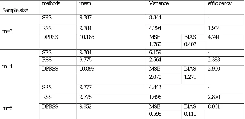
For the performance of mean estimation using a collection of real data set, which consists of the olive yield of each of 64 trees(for more details see Al-Saleh and Al-Omari (2002)). In this study, balanced ranked set sampling is considered. All the sampling done without replacement using the statistical programming 'R'. we obtained the mean and variance of sample mean using SRS, RSS, DPRSS technique using sample size m=3,4,5. We compare the averages of 70,000 sample estimate.

Let,tibe the olive yield of the ith tree i-1,2,...,64. The mean



, and the variance

2



of the population, respectively, are ,









64

1

/

766

.

9

64

1

i

i

kg

tree

t













64

1

2 2

2

/

114

.

26

)

(

64

1

i

i

kg

tree

t





The skewness of the population is 0.475, indicates positively skewed ,i.e., asymmetrical distribution. Hence, we have to find out

)

(

X

_DPRSS(2)

[image:10.612.75.540.305.532.2]

MSE

and efficiency values of

X

_RSS(2) and

X

_DPRSS(2) relative to

X

_SRS(2) for m=3, 4, 5.

TABLE 2: The efficiency values of RSS and DPRSS relative to SRS with sample size m=3,4,5

On the basis of above table, the DPRSS mean at any stage is close to the population mean 9.766, and there is a bias along with MSE as it is a asymmetrical distribution. Hence, DPRSS is much more efficient than SRS, RSS.

VII. SAMPLING WITH ERROR IN RANKING

In RSS, sampling mean is unbiased estimator of population mean without any proper information that, whether it is perfect or imperfect. Hence, it has a smaller variance as compared with SRS having same sample size. So Muttalak(2003) showed that QRSS with error in ranking is unbiased estimator of population mean with assumption that population is symmetric about its mean. Hence applying the above with DPRSS method in ranking with error may be defined as follows,

 

  (2)iqm 1;m

(2) m ; 1 m p

i

and

Y

Y

Let

_  be the first and lastjudgement double partitioned value ofith sample (i=1,2,...,m) having errors

in ranking.Then using DPRSS technique, the estimator of population mean with error in ranking canbe represented as

)

(

1

ˆ

1 1 1

) 2 (

)) 1 ( ( )

2 (

)) 1 ( ( )

2 (

 



  









r

k l

i

m

l i

k m q i k

m p i

DPRSSE

X

X

mr

Y

e , l = m/2

Sample size

methods mean Variance efficicency

m=3

SRS 9.787 8.344 -

RSS 9.784 4.294 1.954

DPRSS 10.185 MSE BIAS 4.741 1.760 0.407

m=4

SRS 9.784 6.159 -

RSS 9.775 2.564 2.383

DPRSS 10.899 MSE BIAS 2.960 2.070 1.271

m=5

SRS 9.777 4.843 -

RSS 9.775 1.696 2.870

DPRSS 9.852 MSE BIAS 8.061

) 2 (

ˆ

e

DPRSS

Y

=

ˆ

1

((

)

₍(2)_{1)[( 1)/2]}

)

1 1 2

) 2 (

)) 1 ( ( )

2 (

)) 1 ( ( )

2 (

k m h r

k h

i

m

h i

k m q i k

m p i

DPRSSO

X

X

X

mr

Y

e  

   











_{ }

_

, h= (m-1)/2

The estimator of population mean µ in ranking with error having following properties,

) 2 (

ˆ

e

DPRSS

Y

with ranking in error is unbiased estimator of population mean with assumption that population is symmetric about its mean.

Var(

ˆ

(2) e

DPRSS

Y

) <Var (SRS) for symmetric distribution and for asymmetric distribution about its mean, MSE(

ˆ

(2)

e

DPRSS

Y

) <Var(SRS) for ranking in error.

The above properties can be proved based on Takahasi and Wakimottto(1968), Dell andClutter (1972), Muttalak (2003) and Al-saleh and Al-kadiri(2000).

VIII. CONCLUSION

In this article, it is observed that, the estimator of proposed Double Partitioned Ranked Set Sampling (DPRSS)is unbiased for population mean and is more efficient than SRS,RSS in case of Symmetrical distribution. From NPR analysis, it isfound that there is greater efficiency with smaller bias in case of estimating of population mean using DPRSS method for asymmetrical distribution. Again, using relative saving method, DPRSS has Greater RS as Compared with RSS.

REFERENCES

[1] Al- Saieh, M.F. and Al-Kadiri, M. (2000). Double ranked Set Sampling. statist. Probab.Lett., 48, 205-212

[2] Dell, T.R. and Clutter, J.L. (1972). Ranked Set Sampling theory with order statistics background.Biometrics 28, 545 -555.

[3] McIntyre, G.A.(1952). A method of unbiased selective sampling, using Ranked sets. Australian Journal of Agriculture Research 3, 385-390 [4] Muttalak, H.A. (1997). Median Ranked set Sampling. Journal of Applied Statistical Science 6, 245-255

[5] Samawi, H.M. (2011) Varied Set size ranked Set sampling with applications to mean and ratio estimation. International Journal of modelling and simulation 31, 6-13.

[6] Strokes, S.L.. (1995). Parametric ranked set sampling. Annals of the Institute of Statistical Mathematics 47, 465- 482

[7] Takahasi, K. and Wakimoto, K. (1968). On unbiased estimates of the population mean based on the sample stratified by means of ordering. Annals of the institute of Statistical Mathematics 20,1-31.

APPENDIX

A. Corollary-1:

Let Xijbe the values assumed by the r.v. X, having probability density function f(X)(x) and cdf F(X)(x) with mean and variance µ and σ2 respectively. A sample of size m was selected and ranked. Let X(1)s,m be the sth smallest rank of the sample, where s=1,2,...,m.

Then mean of X(1)s,mwill be F-1[α(s)]and variance will be

2

) 1 (

,m s



.

Proof:

Let Xijbe a random variable having mean µ and variance σ2 respectively and random sample of size m was selected and ranked.

Let,xs : m =Sth smallest value of the sample where S = 1, ...m, Then pdf and cdf of Xs : m are

 



s

,

m

s

1



F

 

x



1

F

 

x



f

 

x

B

1

x

s 1 m s

,

 









f

_sm

 

x

F

B



F

 

x

;

s,

m

s

1



F

_s:m







respectively.

Where FB (F (x) ; S, m – s + 1) follows a beta distribution function with parameters (S, m – S + 1)

Let

μ

(1)s:m



mean

of

X

(1)s:m

and

σ

s:m

variance

of

X

(1)s:m

respective

ly

2

(1)



,





_

 



 





(1)s;m _s:m 1s;m _s m

; s (1)

P

F

;

dx

x

f

.

x

μ

X

E

and,

F

_s:m

 

x



F

B



F

 

x

;

s,

m



s



1





P

_s

 

s m ; s 1 m ; s (1)

P

F

μ







 



s



F

1







where

 

s



PB



P

s

;

s

.



m



s



1







is an partitioned function for beta distribution with ps=s/m+1

Similarly,

 

x

FB



F

 

x

:

m

s

1

.

s



F

_ms1;m







= qs

 

_s

m : 1 s m 1 m ; 1 s m (1)

q

F

μ





 



=

F

1



PB



q

_s

;

m



s



1,

s





=

F

1



1





 

s



where,

PB



q

s

;

m



s



1,

s





PB



1



P

s

;

m



s



1,

s



= 1- PB( Ps :s, m-s+1)

=

1





 

s

_{and ps + qs= 1}

If f (x) follows symmetrical distribution for any

0





 

s



1

Then



q

_s



μ



μ



P

_s

 



1

s



μ

μ

F



 

s



F

1 1



















 



1

s



F



 

s



2

μ

F

1





1





 





μ

2

μ

μ

(1)s;m



(1)m s1;m







The variance of Xs ; m is given by





 









σ

(1)2s;m

x

μ

(1)s;m 2

f

_s;m

x

dx





 













_s;m (1) s;m 2 2

μ

μ

-dx

x

f

μ

x









_







 





σ

(1)2s;m

μ

(1)s;m

μ

2

x

μ

2

f

_s;m

x

dx













 





















F

(

)

1

F

x

(

)

dx

1

s

m

;

s

B

1

μ

x

2 s 1

x

m s

f

x

<ʃ (x -µ)2f(x) dx = σ2





2 2

m : s (1) m ; s (1)2

σ

μ

μ

σ









as

 



 





s,

m

s

1



1

B

x

f

1

x

F

s 1 m s













The variance of Xs:m may also represented as

 



 































 

du

.

u

1

u

1

s

m

s,

B

s

F

u

F

σ

s1 m-s

2 1

1

m ; s

(1)2



 



 































 

du

.

u

1

u

1

s

m

s,

B

s

F

u

F

σ

s1 m-s

2 1

1

m ; s

(1)2









 





























 

du

.

u

1

u

s

1,

s

m

B

s

-1

F

u

-1

F

m s s-1

2 1

1



m ; 1 s m (1)2

σ





B. Corollary -2

Let

X

(2)s;mbe the sth smallest value of a random sample of size m. The sample was selected from a population having probability

density function f(1)s,m(x) and cdf F(1)s,m(x) with mean and variance

) 1 (

,m s



and



_s(1_,m)2 respectively. After ranking a size of m sample was selected and let x (2)s,m be the sth smallest rank of the sample, where s=1,2,...,m. Then mean ofX(2)s,mwill be F-1[α.α(s)]and

variance will be



_s(_,2_m)2. Proof:

Let X(2)ijbe a random variable from population having mean µ and variance σ2 respectively

When a random sample from population of size m was selected and ranked. Let, X(2)_{s : m =S}th smallest value of the sample where S = 1, ...m,

Then pdf of population is

 



s

;

m

s

1



F

 

x



1

F

 

x



f

 

x

B

1

x

f

(1)s;m _s,ms 1 m s _s,m

m s,

 









where, the mean and variance of

x

_ij(1)are µ(1)and σ(1)2 respectively.

and also let

x

(2)m-s1;m be the (m – s + 1)th smallest value

Then







































  



  



m ; 1 s m (2) m ; 1 s m (2)

m ; s (2) m ; s (2)

m ; 1 s m (2) m ; 1 s m (2)

m ; s (2) m ; s (2)

2 2

σ

x

V

σ

x

V

μ

x

E

μ

x

E

Then,

 



α

s



F

μ

(2)s:m



1s;m

 





*s

, 1

P

s

α

.

α

F







m

s

again,

μ

(2)ms1;m



F

1s;m



1



α

 

s



=

F

s,m1



1





.



(

s

)





s *

q



For symmetric distribution for 0 ≤α ≤ 1

* s s

*

P

μ

μ

q









 



1

α

.

α

s



μ

μ

F



α

.

α

 

s



F

1









1



 



1

α

.

α

s



F



α

.

α

 

s



2

μ

F

1 1









 

μ

2

μ

μ

(2)m s 1;m



(2)s;m



The variance of X (2)s:m will be





 







x

μ

f

x

dx

σ

s;m

2 m ; s (2) m ; s (2)2





 





2

m ; s (1) m ; s (2) m ; s 2 m ; s (1)

μ

μ

dx

x

f

μ

x









_





(1)2s;m 2 m ; s (1) m ; s (2) m ; s (2)

σ

μ

μ

σ

2









as

_







_s;m

 



(2) s;m 2 m ; s (1) 2

σ

dx

x

f

μ

x





(1,)2

2 ) 2 (

,m sm s





Again



 







2

, 2 m ; s (1) m ; s (1)2 2 m ; s (1) 2 m ; s (1) m ; s (2) m ; s (2)

μ

μ

σ

μ

μ

μ

μ

σ

2



















_sm



)

var(

)

var(

)

var(

DPRSS



RSS



SRS



The variance of X(2)s:m may also represented as

 



 





























u



1

u

.

du

1

s

m

s,

B

s

F

u

F

σ

s 1 m-s

2 1 -(1) m s, 1 -(1) m s, m ; s (2)2



For symmetrical f (x),

 



 





























_u



₁

_u

_.

_du

1

s

m

s,

B

s

F

u

F

σ

s1 m-s

2 1 -(1) m s, 1 -(1) m s, m ; s (2)2









 



























 

du

.

u

1

u

s

1,

s

m

B

s

.

F

u

-1

F

m s s-1

2 1 -m s, 1 ) 1 ( m

s,











 



























 

du

.

u

1

u

s

1,

s

m

B

s

.

-1

F

u

-1

F

m s s-1

2 1 1 -(1) m

s,











 



























_u



₁

_u

_.

_du

s

1,

s

m

B

s

-1

F

u

-1

F

_s,(1)_m-1 _s,(1)_m-1



2 _{m s s-1}

m ; 1 s m (2)2

σ





C. Corollary-3

1. DPRSS

) 2 (





is an unbiased estimator of the population mean, for givenassumption that population is symmetric about its mean. Proof :

For kth cycle and ith sample,

D. If m is even,

 

 



x

(2)1 p m1 k

.

x

(2)2pm1k...

x



p



m

1





k

x

(q



m

1



k,

x

(2)

(q

(m

1)

k

2 2 m ) 2 ( 1 2 m (2) 2

m





















  ...







q

m

1



k





_{   }





















_

_

     m 1 j m ; 1 s m j ) 2 ( 1 i m ; s i ) 2 ( DPRSSE (2

x

x

m

1

μ

 







 





 



_





















_

_

     m 1 j m ; 1 s m j (2) 1 i m ; s i ) 2 ( DPRSSE (2)

x

E

x

E

m

1

μ

E

     

















(2)s;m

μ

(2)ms1;m

2

m

μ

.

2

m

m

1



μ

(2)s;m

μ

(2)m s 1;m



2

m

m

1

 







μ

2

2

1







μ

E. If m is odd,[

x

(2)1(p(m1)k),

x

(2)2(p(m1)k)...

k) 1) (m (p 2 1 -m (2)

x

 ],[ 1((m1)/2)k 2 1 -m ) 2 (

x



 ],[ 2(qm 1k

2 1 -m ) 2 (

x

  ,...,

m 1k) (q 3 2 1 -m (2)

x



 ... m(qm 1k)

(2)

x

 ]is the sample of size DPRSSO.



   























      





2 1 )( 1 2 1 -m ( m 2 h j m ; 1 s m j (2) h 1 i m ; s i (2) DPRSSO (2)

x

x

x

m

1

μ

ˆ

_m







 





 































     





;m

2 1 m (2) m 2 h j m ; 1 s m j (2) n 1 i m ; s i (2) DPRSSO (2)

X

E

X

E

x

E

m

1

μ

ˆ

E



μ

μ



μ

μ

2

1

m

m

1

m ; 1 r m (2) m ; s (2)























 

Hence,

μ

ˆ

(2) _DPRSS is an unbiased estimator of the population mean.

F. Corollary-4

Var



X

DPRSS



is less than each of Var



X

_SRS



and Var



X

_RSS



.

Proof :

For m is even, Then Variance will be









 





(2)im s 1;m



m 1 2 m j 2 m ; s i ) 2 ( m/2 1 i 2

DPRSSE

var

X

1

var

m

1

μ

ˆ

var

 

  





_



















m

X





m

σ

σ

σ

m

2

1

, (2)2

m ; 1 s m (2) m ; s

(2)2 2 sm







 

)

var(

)

var(

)

var(

DPRSSE



RSS



SRS



Then Variance can be defined as

















 





























 

 









(2)jm s 1;m

m

2 1 m i m . 2

1 m (2) 1/2

m

1 i

m ; (s i (2)

DPRSSO

var

X

var

X

var

X

m

1

μ

ˆ

var































m ; 2

1 m (2) (2)

m ; s (2) 2

2 2

2

σ

m

;

1

s

m

σ

σ

2

1

m

m

1

)

)

2

(

2

1

(

1

(2)2

, 2 ) 2 (

,

2 sm sm

m

m











2 ) 2 (

,

1

m s

m







D

P

R

S

SO



var



R

S

S



var



S

R

S



var



