Technology (IJRASET)
Impulse Noise Reduction and Enhancement of
Gray Scale and Color Images
CH.V.Nagendra Babu1, N.Pushpaltha2, B.Neelima3 M.Tech(DECS) Student, Assistant professor, Assistant professor
Department of ECE, AITS, Annamacharya Institute of Technology and Sciences, Tirupati, India
Abstract—A new filtering algorithm, adaptive weight algorithm, is developed for the removal of impulse noise present in the Images. This approach has two major steps, in that, first is to detect noise pixels according to the correlations between image pixels, and then use different techniques based on the various noise densities. Adjacent signal pixels mean method was adopted for the low noise density, to reduce the noise in image, for the high noise density, adaptive weight algorithm was adopted. Experiments shown that the proposed algorithm has advantages over standard methods in terms of both edge preservation and noise reduction, and even for high density image with noise level as high as 90%, this method still can get a significant performance.
Keywords: Impulse noise; adaptive weight algorithm; adjacent signal pixels mean method; high density image.
I. INTRODUCTION
Images captured by cameras may produce noise due to malfunction of camera pixels. And these captured images often were polluted by various noises during the course in which they are generated or transmitted. Due to which the quality of the image will be damaged. The disturbance is most likely the noise in the digital images and this is generated due to the transmission of an image. We have different types of noises like Gaussian noise, spike noise or impulse noise etc. Impulse noise is also called salt and pepper noise[1]. The most well-known type of the noise in images is the salt and pepper noise. It is the noise, which, sprinkles on the images like white (salt) and black (pepper) dots significantly reduces the visual effects of images. Wiener filtering algorithm and median filtering algorithms, are the two most used algorithms, to remove impulse noise present in the digital image. But, the regular filtering algorithms are not effective to remove the noise, especially for high noise densities. To reduce the high level noise density and to improve the quality of image, it is very important to keep the margins (edges) and details, as well as, removing noises pixels in images.
We have different regular methods for the removal of impulse noise. Among all the common impulse noise filtering algorithms: Traditional Median (TM) filter algorithm; Switching Median (SM) filter algorithm [2], and Adaptive Median (AM) filter algorithm etc [3][4] are the good known algorithms;. TM (Traditional Median) filter algorithm is simple and speed, but it does not have the ability of effectively removing salt and pepper noise and protection for edges and details in high noise density case [5].
SW (Switching Median), and AM (Adaptive Median) filter algorithms are sensitive to different noise density levels, as their filtering properties get worse with the increase in the noise density. For high density noise levels [6], decision-based median filtering algorithms are used. These methods first identify noisy pixels and then replace them with appropriate estimates using neighbor pixels value, but noisy pixels present in the image are not effective to detect and estimate replacing pixel. In [7], an Adaptive Weight (AW) approach was used, in which the output is a weighted sum of the image and a de-noising factor. And these weighting coefficients depend on a state variable of the neighboring pixels of the image. The state variables are the difference between the current pixel and the average of remaining pixels in the surrounding window of a particular portion of the image. Due to the presence of the various coefficients, it is very difficult to choose an appropriate one.
Technology (IJRASET)
©IJRASET 2014: All Rights are Reserved
500
Fig1. Switching adaptive weight filtering algorithm schematicAmong the two, Signal pixels are kept same and only the noise pixels are processed. And in second block, filtering block, different approaches were taken according to the noise density levels. In the low level noise density case, adjacent signal pixels mean method is selected. While in the high noise density level, the proposed adaptive weight algorithm is used.
II. OVERVIEW OF NOISE AND FILTERING A. Image Noise
The main source of noise in digital images arises during image transmission. For instance, an image transmitted over a wireless network might be corrupted as a result of lighting or other atmospheric disturbance. The image noise is random (not present in the object image) variation of brightness or color information in digital pictures (images), and is usually an aspect of electronic noise. The probability density function is given by equation from the above equation, Bipolar if neither Pa nor p is zero. Bipolarone, also known as salt-and-pepper, impulse and spike noise. It is called unipolar if either p or p is zero. An image containing impulse noise will have dark pixels in bright regions and bright pixels in dark regions.
p(z) =
p for z = a p for z = b 0 otherwise
Image noise is a random variation of brightness or color information in images, and is usually an aspect of electronic noise. Digital Image processing is an Electronic Domain in which image is divided into small unit called pixel and subsequently various operation has been carried out on the pixels. Noise can be usually originated in the sensor or transmission channel during the acquisition and transfer procedure for the digital signal images. In the Digital Image Processing field, removing the noise from the image is the critical issue.
In past years, linear filters became the most popular filters in image signal processing. The reason of their popularity is caused by the existence of robust mathematical models which can be used for their analysis and design. The benefit of nonlinear filters lies in their ability to preserve edges and suppress the noise without loss of details. The success of nonlinear filters is caused by the fact that image signals as well as existing noise types are usually nonlinear. As salt and pepper noise is a random valued shot noise, it is very difficult to remove this type of noise using linear filters. Median filters are non-linear. In this paper we compared the proposed adaptive weight algorithm experimental results with the wiener filter and the median filter. And PSNR and MSE versus Noise plots are also compared with the proposed adaptive weight algorithm.
B. Noise Filtering methods and process
We have different types of noise filtering methods used in the, digital image processing, de-noising of the noise present in image. But the noise filtering algorithms can be classified based on how filtering is applied to noise image. Noise filtering classified as spatial filtering and order statistics filtering. The filtering methods come under the spatial filtering is only employed when random
noise is present. Arithmetic mean filter, Geometric mean filter, Harmonic mean filter, and Contra harmonic mean filter are the
filtering techniques used in spatial filtering.
Fig2. Noise Filtering
Technology (IJRASET)
values of the pixels contained in the filter window. Median filter, Max and min filters, Midpoint filter, and Alpha-trimmed mean filter are the filters come under order statistics filtering.In Digital image processing, Wiener filter is used to produce an estimate of a desired or target random process by linear
time-invariant filtering of an observed noise present in an image, assuming known stationary signal and the noise spectrum, and the
additive noise. And, also, he Wiener filter minimizes the mean square error between the estimated random process and the desired
process. The main aspect of the Wiener filter is to filter out noise that is present and corrupted the image. It is based on the ordered
statistical approach.
In digital image processing, always it is required to be able to perform some kind of noise reduction on an image. Median filtering is
very widely used in digital image processing, because it preserves edges while removing noise. In general the image with noise is
given to the filtering algorithm that best suited to remove the type of noise ex. impulse present in the given image. And the adopted filter performs the filtering operation on the given image and gives the image with reduced or removed noise, the noise filtering operation process steps are shown in fig2.
C. Impulse noise model and definitions
In different types of salt and pepper noise models, for images, the noised pixels are sometimes replaced with the values of pixels nearest or equal allowable minimum or maximum window. Typically this corresponds to fixed values near 0 or 255 for the 8 bit images. Let consider a, general, a noise model in which a noisy pixel can take on arbitrary values in the dynamic range according to underlying probability distribution function. Let assume that v(n) and x(n) be the luminance values of the original image and noisy
image respectively. And now the impulse noise model with error probability , then we have
( ) = ℎ ℎ 1 −
Where is independent random process with arbitrary probability density function. We generate corrupted impulse noise
described by a uniform distribution from 0 to 255.
Fig3. Elements of sliding window (3x3) around a pixel ( ).
Now consider a real valued 2D sequence
( ) and it is defined as an 8 bit element observation vector. The mean of the ( ) pixel can be calculated from the surrounding 8 pixels. And is given by the average of the all surrounding eight pixels of the pixel ( ).
III. PROPOSED FILTERING ALGORITH
Let I be the preprocessing image and whose size is M x N. xi,j be the gray value of the pixel at location (i, j), and δ be the threshold
used to decide whether the pending pixel belongs to noise pixels or not, fi,j be the values of the label matrix at pixel location (i, j)
which is defined by:
, =
1 255 − ≤ , ≤ 255
−1 (1)
It is known that the salt and pepper noise’s value is the max or min value in the image according to the characteristic of the noise sprinkling on images. If , = 0, it means the pixel is a signal point, else it is a noise one. Because the values of some signal pixels are absolutely around 0 or 255, it I needed to further decide whether the pixel I a noise one or not. After 40 images experiments, we find that it I advantage to use the temple window whose size is 5x5 to the noise detection, so as the paper.
( ) ( ) ( )
( ) ( ) ( )
Technology (IJRASET)
©IJRASET 2014: All Rights are Reserved
502
If , (| , | and s.t≠ 0) are not all zero, it means that there are some signal pixels in the temple window centered at (i+s, j+t).
Let T be the threshold and , be the mean value of signal pixels but the center pixel itself in the temple window. Compare the D-value between , and , with T. If , − , >T, the pixel is regarded as a signal point, else it is a noise one.
, = , , − , >
0 (2)
If , (| , | ≤ 2 and s.t≠ 0) are all zero, it means that there are all probable noise pixels in the temple window. Let m and n be
the number of salt and pepper noise in it separately. If , belongs to the larger number one of salt and pepper noise, the pixels is regarded as a signal point, else it is a noise one.
, =
0 > , = 1 < , = −1
, (3)
Noise Filtering:
The signal pixels are kept the same and only the noise pixels are corrected. Different methods should be adopted for various noise densities. The specific steps as follows:
(1) Preliminarily estimate the noise density of the preprocessing image.
= (4)
(2) When p is less than 30%, it is advantage to adopt the method of adjacent signal pixel mean value because of many signal pixels around the noise pixels. Let be the temple window of size 3x3 centered at (i,j) and , be the mean value of all the signal pixels but the center pixel itself in . If , =0, , is kept the same, else , will be substituted by , .
, =
, , ≠ 0
, , = 0 (5)
When p is more than 30%, if , = 0, , is kept the same, else compute the signal pixel’s number marked as in . If =0, it means that they are all noise pixels in , then move the window center to the next noise pixel. If ≠ 0, it means there are some signal pixels in . First compute the D-value between (| , | ≤ 1 and a.b = 0) and , , then compute their inverses marked as
, :
, = , , = 0
0
(6)
Because of the correlations between image pixels depending on their spatial location relationship, generally, the closer the distance between the two pixels are, the higher the correlations of them are. So it can make full use of spatial location relationship between the neighborhood pixels position weight marked as , :
, =
0 = = 0
0.25 | | = | | = 1 0.5
(7)
Let , be the initial weight coefficients, , be the normalization weight coefficients.
T= , X , (8)
, = ∑ ∑ ,
, (9)
Technology (IJRASET)
, = ∑ ∑ , , (10)
, Will be substituted by , and the pixel will be regarded as a signal point later.
, =
, , ≠ 0 = 0
,
(11)
, = ,
= 0
0 ≠ 0 (12)
As getting the restored image marked as I 2, we check whether there is some noise in I 2or not. If there is still some noise in it, the image I 2 will be regarded as the raw input image I and the step 3 will be repeated until there is no noise in it. Then the loop is terminated.
IV. SIMULATION AND ANALYSIS A. Gray scale image
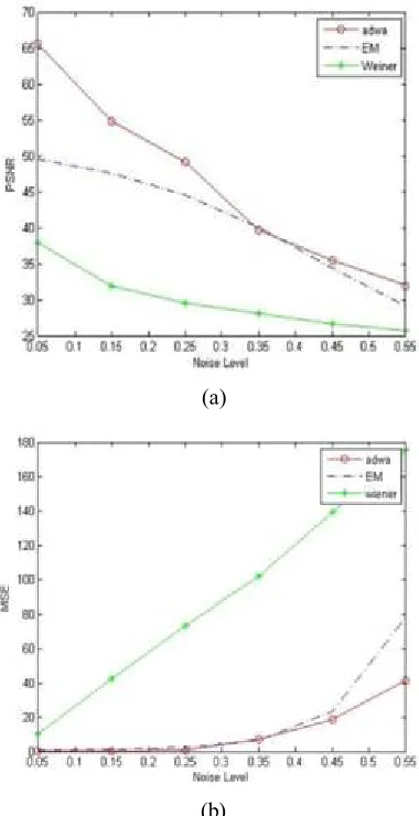
To verify the advantage and effectiveness of our filtering algorithm, a gray scale image whose size is 256 x 256 was selected. Now the salt and pepper noise was added to the image. Then EM (Extreme Median), Wiener filter and our algorithm were used, separately, to restore the image corrupted by salt and pepper noise. Fig.5. is the visual results comparison of different methods. Fig6(a). is the image Peak Signal to Noise Ratio (PSNR) versus noise comparison of our method with different algorithms at various noise ratios for the test image. The results of all three algorithms shows that: Wiener filter is applicable for the situation of the very low noise density. And the extreme median filtering algorithm shown best results for low noise and medium levels but as the noise levels increases the extreme median is more similar to wiener filter. Based on the noise signal strength of the image, our method considers that one of the best methods we used in the algorithm. If noise density less than thirty percent, then adjacent signal mean pixel value algorithm chooses, otherwise if noise density greater than thirty percent then the adaptive weight algorithm will be chosen.
Supposing , and , are separately the gray scale values of the original image and the output image at the pixel location (i,j). The image size is MxN, PSNR is the image peak signal to noise ratio.
=
∑ ( , ,) (13)
Compared with the filtering results of TM, EM, and the proposed algorithm, we can see that the PSNR of the proposed algorithm is best at different noise densities situation. It shows that the restored result of the proposed algorithm is best at different noise density situation. When the noise density is more than 60%, other filtering algorithm PSNR drops off precipitously.
(a)
(b)
Technology (IJRASET)
©IJRASET 2014: All Rights are Reserved
504
10% Noise (A) (B) (C)
25% Noise (A) (B) (C)
50% Noise (A) (B) (C)
75% Noise (A) (B) (C)
90% Noise (A) (B) (C)
Technology (IJRASET)
With the noise density improving, the difference value between the proposed algorithm and the other algorithms is larger especially when the noise density is up to 90%, their PSNR difference value is about 10 db. Experiments shows that the proposed algorithm has better de-noising and protection detail capacity.(a)
(b)
Fig 6. (a) PSNR vs Noise and (b) MSE vs Noise Plots
From above figure 6(a), we can clearly see that, as the noise increases the PSNR of the output image is also increased. So, clearly, the PSNR of the proposed algorithm over noise is much greater than the other, two methods, wiener filtering and the extreme median filtering. So that we can clearly say that the proposed algorithm is more useful than the other counter parts. Similarly from fig 6(b), we can see that the proposed algorithm has low MSE as the noise increases, while the extreme median filtering and the wiener filtering has high MSE as noise increases. So we can say that the proposed algorithm is performing well at high noise density levels.
B. Color Image
[image:8.612.209.399.146.516.2]Technology (IJRASET)
©IJRASET 2014: All Rights are Reserved
506
(a)
(b)
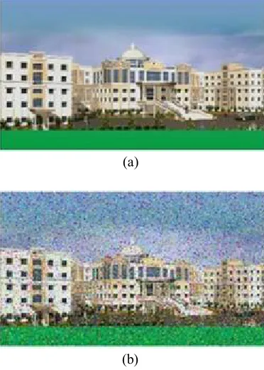
Fig 7. (a) input image (b) Image with Impulse noise
In this method we first take RGB color image, by using the imread( ) function. And we know that in an RGB color image is a combination of red, green and blue channels. So, now the individual red channel, green channel, and the blue channels will be extracted from the given RGB input image. After extracting the red, green, and blue channels, now, for
70% Noise Restored Image
[image:9.612.214.400.115.376.2]90% Noise Restored Image
[image:9.612.106.473.454.704.2]every individual red, green, and blue channels. The reduced impulse noise or salt and pepper noise images of the individual channels are then combined together to form an RGB color image output. Results are shown in Fig.8
V. CONCLUSION
An efficient filtering algorithm is proposed for filtering the salt and pepper noise at different noise density levels. First to detect noise density and then different techniques are applied to various noise densities. Experimental results shows that this algorithm can suppress the noise effectively. Especially for the high noise density levels, the proposed algorithm has more obvious advantages. For suppressing the noise in a color image, first we converted the RGB image into red, green, and blue channels. And filtering is performed on each channel. Finally the noise suppressed individual channels are combined to get the desired de-noised RGB color image.
REFERENCES
[1] T. Sun and Y. Neuvo, Detail-preserving median based filters in image processing, Pattern Recognition Letters, vol. 15, no. 4, 1994, pp. 341–347.
[2] Z. Wang and D. Zhang, Progressive switching median filter for the removal of impulse noise from highly corrupted images, IEEE Transactions on Circuits and Systems-II, vol. 46, 1999, pp.78–80.
[3] H. Hwang and R. A. Hadded, Adaptive median filter: new algorithms and results, IEEE Transactions on Image Processing, vol. 4, no. 4, 1995, pp. 499–502. [4] J. Astola and P. Kuosmaneen, Fundamentals of Nonlinear Digital Filtering Techniques. Boca Raton, FL: CRC, 1997.
[5] S. Zhang and M. A. Karim, A new impulse detector for switching median filters, IEEE Signal Processing Letters, vol. 9,no. 11, 2002, pp. 360–363.
[6] R. H. Chan, C.W. Ho and M. Nikolova, Salt-and-pepper noise removal by median-type noise detectors and detail preserving regularization, IEEE Transactions on Image Processing, vol. 14, no.10, 2005, pp. 1479–1485.
[7] P. E. Ng and K. K. Ma, “A switching median filter with boundary discriminative noise detection for extremely corrupted images,” IEEE Trans. Image Process., vol. 15, no. 6, pp. 1506–1516, Jun. 2006.
[8] V. Jayaraj and D. Ebenezer, “A new switching-based median filtering scheme and algorithm for removal of high-density salt and pepper noise in image,” EURASIP J. Adv. Signal Process, 2010.
[9] R. C. Gonzalez, and Woods R.E, Digital Image Processing. Addison-Wesley, Boston, 2005.
[10] K. S. Srinivasan and D. Ebenezer, “A new fast and efficient decision based algorithm for removal of high density impulse noise,” IEEE Signal Process. Lett., vol. 14, no. 3, pp. 189–192, Mar. 2007.
[11] Zhu, Rong, and Yong Wang. "Application of Improved Median Filter on Image Processing." Journal of Computers 7, no. 4 (2012): 838-841.
AUTHOR DETAILS
Mr. CH.V.NAGENDRA BABU received the B.Tech Degree in E.C.E from Malinenei Lakshmaiah Institute Of Engineering and Technology (JNTU ANANTAPUR), Nellore, Andhra Pradesh, India in 2012. He is pursuing his M.Tech Degree at Annamacharya Institute of Technology and Sciences (AITS) Tirupati. His area of interest includes digital image processing, Electronic devices and circuits, Networks Analysis, and digital systems.
Ms. B.NEELIMA completed her B.Tech at Gokula Krishna college of Engineering(JNTU Anantapur), Sullurpet, Andhra Pradesh, India in 2006 and M.Tech at JNTU college of Engineering, Anantapur in 2013. Presently she is working as Assistant Professor of ECE, Annamacharya Institute of Technology and Sciences, Tirupati. Her Research area includes digital image processing.