How Would 401(k) ‘Rothification’
Alter Saving, Retirement Security,
and Inequality?
Vanya Horneff, Raimond Maurer, and Olivia S. Mitchell
How Would 401(k) ‘Rothification’ Alter
Saving, Retirement Security, and Inequality?
Vanya Horneff Raimond Maurer Olivia S. Mitchell
Finance Department, Finance Department, Wharton School,
Goethe University Goethe University University of Pennsylvania
September 2019
Michigan Retirement and Disability Research Center, University of Michigan, P.O. Box 1248. Ann Arbor, MI 48104, https://mrdrc.isr.umich.edu/, (734) 615-0422
Acknowledgements
The research reported herein was performed pursuant to a grant from the U.S. Social Security Administration (SSA) funded as part of the Retirement Research Consortium through the University of Michigan Retirement and Disability Research Center Award RDR18000002-01. The opinions and conclusions expressed are solely those of the author(s) and do not represent the opinions or policy of SSA or any agency of the federal government. Neither the United States government nor any agency thereof, nor any of their employees, makes any warranty, express or implied, or assumes any legal liability or responsibility for the accuracy,
completeness, or usefulness of the contents of this report. Reference herein to any specific commercial product, process or service by trade name, trademark, manufacturer, or otherwise does not necessarily constitute or imply endorsement, recommendation or favoring by the United States government or any agency thereof.
Regents of the University of Michigan
How Would 401(k) ‘Rothification’ Alter
Saving, Retirement Security, and Inequality?
Abstract
The U.S. has long incentivized retirement saving in 401(k) and similar retirement accounts by permitting workers to defer taxes on contributions, levying them instead when retirees withdraw funds in retirement. This paper develops a dynamic life-cycle model to show how and whether “Rothification” — that is, taxing 401(k) contributions rather than payouts — would alter
household saving, investment, and Social Security claiming patterns. We show that these changes differ importantly for low- versus higher-paid workers. We conclude that moving to a system that taxes pension contributions instead of withdrawals will lead to later retirement ages, particularly for the better-educated. It also would reduce work hours and lifetime tax payments and increase wealth and consumption inequality. In addition, we show how these behaviors would differ in a persistently low interest rate environment versus a more “normal” historical return world.
Citation
Horneff, Vanya, Raimond Maurer, and Olivia S. Mitchell. 2019. “How Would 401(k)
‘Rothification’ Alter Saving, Retirement Security, and Inequality?” Ann Arbor, MI. University of Michigan Retirement and Disability Research Center (MRDRC) Working Paper; MRDRC WP 2019-398. https://mrdrc.isr.umich.edu/publications/papers/pdf/wp398.pdf
Authors’ acknowledgements
The authors acknowledge research support for this work from the Michigan Retirement and Disability Research Center (MRDRC), the German Investment and Asset Management
The United States has long incentivized retirement saving by deferring taxes on workers’ pension contributions until the assets are withdrawn in old age, at which point the withdrawn funds become subject to income tax. In this way, most 401(k) retirement accounts are taxed according to an “EET” regime: Workers contribute out of pretax earnings, recognize pretax investment earnings in their accounts, and pay income tax on withdrawals during retirement. This policy has a large current budgetary cost: the U.S. Treasury foregoes over $100 billion per year due to tax-deferred contributions to 401(k) and similar plans (Thornton 2017).1 Partly because of projected federal budget
shortfalls, some policymakers have recently proposed eliminating or capping tax-qualified retirement plan contributions, a practice termed “Rothification,” named after Senator William Roth who successfully passed legislation allowing this in 1997. Specifically, the idea would be to treat all future retirement contributions to a “TEE” regime, in which workers would contribute to their pensions out of after-tax income, and then no additional tax would be levied thereafter (Schoeff 2017).
The Rothification idea has been a topic of considerable recent discussion, with former President Obama recommending a pretax pension contribution cap in 2015, and related proposals offered by the Trump Administration during the 2017 tax-reform debate. Though those proposals were not enacted, the topic is certain to be revisited given the amount of revenue involved. In an economy with a single tax rate and a flat benefit system, taxing benefits now versus later is unlikely to change behavior. Yet in the
U.S. economy, there are numerous nonlinearities in the tax and Social Security systems that render less obvious the ways in which such a reform might alter household
behavior. Accordingly, if such a reform were to be passed in the future, it could have important implications for household behavior. Moreover, effects are likely to vary across different population subgroups.
To date, however, there has been no coherent microeconomic analysis of how Rothification could alter household consumption, saving, retirement patterns, and tax-payments. Our paper fills this gap by developing a richly detailed and state-of-the-art life-cycle stochastic dynamic model with endogenous work effort, portfolio choice, consumption, saving, and Social Security claiming patterns, to evaluate such a policy’s potential effects for the population overall and for different population subgroups. Of key importance is heterogeneity: That is, how outcomes will differ for workers with different lifetime earnings profiles. For instance, some have argued that “Roths may not, in fact, work out to be a better deal” for low-income people (Tergesen 2017), while others argue the opposite.2 We therefore assess how key outcomes change for a variety of
worker-types differentiated by sex and education.
Additionally, it is important to recognize that converting retirement plans to Roth plans would take place against the backdrop of the new income tax structure
implemented in 2018, which reduced the tax burden for most earners.3 The tax reform,
therefore, also changed the relative attractiveness of saving for retirement in an EET
2 Hallez (2017) reports that some predict that low-wage workers would save less in a TEE regime, whereas Statman (2017) concluded the opposite.
environment, since lower marginal tax rates on workers’ earnings decreased the attractiveness of saving in 401(k) accounts. Our research also compares how work, saving, benefit claiming behavior, and tax payments would respond in an EET versus TEE setting for a heterogeneous set of workers.
Finally, we analyze how our results would differ if the economy were to move out of the very low interest rate environment of the last decade, and return to a more
“normal” regime. We know that persistent low returns spur workers to save and invest differently and can also drive different decisions about how long to work and when to claim Social Security benefits (Horneff, Maurer, and Mitchell 2018). The quantitative easing policies of the U.S. Federal Reserve Bank after the financial crisis have resulted in extraordinarily low real U.S. Treasury yields over the past decade, compared to the normal historical real return of 3% (1989-2008).4 We seek to study how appealing
Rothification might be in this new low interest rate environment, compared to the traditional EET framework, for the $5 trillion invested in 401(k) assets.
In what follows, we first build and calibrate a structural life-cycle model, assuming an EET framework calibrated to U.S. federal/state income tax and Social
Security/Medicare premium structures, and realistic Social Security benefit formulas, including adjustments for early and delayed claiming. Importantly, the baseline model also incorporates real-world rules characterizing EET tax-qualified 401(k) accounts including the current caps on 401(k) pretax contributions, employer matches, penalties and taxes on early withdrawals, and Required minimum distribution withdrawals. We show that our results agree closely with observed consumption, saving, and Social
Security claiming age behavior of U.S. households, while matching the current distribution of 401(k) wealth rather nicely.
Next, we develop results under an alternative environment where 401(k) contributions are taxed according to a TEE structure. This permits U.S. to identify changes in behavior for the heterogeneous workers described above, under the two tax regimes (EET versus TEE).
Next, we compare results with those obtained in a higher real return environment. In particular, we assess whether the lower-paid behave differently from the higher-paid in terms of savings inside and outside the tax-qualified accounts, as well as in
nonpension savings accounts, and whether they would change their claiming behavior for Social Security benefits. In addition, we are interested in how Rothification would alter the distribution of retirement incomes relative to the current EET-system. For example, the gap between high- and low-wage workers’ take home pay is not
payments, reductions in consumption, and higher wealth and consumption inequality. Retirement asset accumulation is also lower under the Rothification regime.
Related literature
This research builds on prior work (Horneff, Maurer, and Mitchell 2018, 2019) by exploring the impact of a Rothification reform for 401(k) plans. Here we add to the literature by delving into the distributional impacts of such a reform in both a “normal” and a low return environment, while accounting for the income tax regime recently adopted. Our work is informed by a number of studies using a life-cycle framework to model and evaluate how individuals respond to a range of environmental shocks. For example, the workhorse model of Cocco, Gomes, and Maenhout (2005) and Gomes and Michaelides (2005) was subsequently extended by Love (2010) and Hubener, Maurer and Mitchell (2016), who showed how family shocks due to changes in marital status and children alter optimal consumption, insurance, asset allocation, and retirement patterns. Horneff, Maurer, Mitchell, and Rogalla (2015) demonstrated how capital market surprises can influence saving and portfolio allocation patterns, and Chai, Horneff,
Horneff, Maurer, and Mitchell (2016), we do not include annuity purchases, but we do allow flexible work effort and endogenous claiming of Social Security benefits.5
The consumer’s life-cycle problem: model and calibration
In what follows, we build and calibrate a structural dynamic consumption and portfolio choice model for an individual maximizing his utility over his life cycle using a richly specified, sophisticated formulation of lifetime behavior calibrated to U.S.
federal/state income tax and Social Security/Medicare premium structures, along with realistic Social Security benefit formulas.6 Just as importantly, the baseline model also
incorporates real-world rules characterizing EET tax-qualified 401(k) accounts including the current U.S. caps on 401(k) pretax contributions, employer matches, penalties and taxes on early withdrawals, and required minimum distribution withdrawal amounts. Results using calibrated baseline parameters agree closely with observed consumption, saving, and Social Security claiming age patterns of U.S. households. Specifically, our model generates a large peak at the earliest claiming age at 62, along with a second peak at the (system-defined) Full Retirement Age. The model also matches the current distribution of 401(k) wealth rather nicely (Horneff et al. 2018).
Preferences
We work in discrete time and assume that the worker’s decision period starts at
𝑡𝑡 = 1 (age 25) and ends at 𝑇𝑇= 76 (age 100). Accordingly, each period corresponds to
5 We also provide a theoretical backing for the empirical claiming age patterns identified by Shoven and Slavov (2012, 2014).
one year. The household has an uncertain lifetime, such that the probability to survive from 𝑡𝑡 until the next year 𝑡𝑡 + 1 is denoted by 𝑝𝑝𝑡𝑡. Survival rates entering into the utility
function are taken from the U.S. Population Life Table (Arias 2010). Preferences are
represented by a Cobb Douglas function 𝑢𝑢𝑡𝑡(𝐶𝐶𝑡𝑡,𝑙𝑙𝑡𝑡) = (𝐶𝐶𝑡𝑡𝑙𝑙𝑡𝑡
𝛼𝛼)1−𝜌𝜌
1−𝜌𝜌 based on current
consumption 𝐶𝐶𝑡𝑡 and leisure time 𝑙𝑙𝑡𝑡 (normalized as a fraction of total available time). The
parameter 𝛼𝛼 measures leisure preferences; 𝜌𝜌 is the coefficient of relative risk aversion; and 𝛽𝛽 is the time preference factor. The recursive definition of the value function is given by:
𝐽𝐽𝑡𝑡 =(𝐶𝐶𝑡𝑡𝑙𝑙𝑡𝑡 𝛼𝛼)1−𝜌𝜌
1− 𝜌𝜌 +𝛽𝛽𝐸𝐸𝑡𝑡(𝑝𝑝𝑡𝑡𝐽𝐽𝑡𝑡+1 ) ,
(1)
with terminal utility 𝐽𝐽𝑇𝑇 =�𝐶𝐶𝑇𝑇𝑙𝑙𝑇𝑇
𝛼𝛼�1−𝜌𝜌
1−𝜌𝜌 and 𝑙𝑙𝑡𝑡= 1 after retirement. We calibrate the preference
parameters so our results match empirical claiming rates reported by the U.S. Social Security Administration and average assets in tax-qualified retirement plans. This
matching procedure produces preference parameters of 𝛼𝛼= 1.2, 𝜌𝜌= 5 and 𝛽𝛽= 0.96 (for details, see below).
Time budget, labor income, and Social Security retirement benefits
As in Horneff et al. (2016), our model allows for flexible work effort and retirement ages. The worker has the opportunity to allocate up to (1− 𝑙𝑙𝑡𝑡) = 0.6 of his available time
budget to paid work (assuming 100 waking hours per week and 52 weeks per year). Depending on his work effort, the uncertain yearly before-tax labor income is given by:
Here 𝑤𝑤𝑡𝑡 is a deterministic wage rate component which depends on age, education, sex,
and an indicator for whether the individual works full time, part time, or overtime. The variable 𝑃𝑃𝑡𝑡+1 =𝑃𝑃𝑡𝑡·𝑁𝑁𝑡𝑡+1 is the permanent component of wage rates with independent
lognormal distributed shocks 𝑁𝑁𝑡𝑡~𝐿𝐿𝑁𝑁(−0.5σP2,σ𝑃𝑃2), having a mean of one and volatility of
σ𝑃𝑃2. In addition, 𝑈𝑈
𝑡𝑡~𝐿𝐿𝑁𝑁(−0.5σU2,σ𝑈𝑈2) is a transitory shock with volatility σ𝑈𝑈2 and assumed
uncorrelated with 𝑁𝑁𝑡𝑡.
The calibration of the deterministic component of the wage rate process 𝑤𝑤𝑡𝑡𝑖𝑖 and
the variances of the permanent and transitory wage shocks 𝑁𝑁𝑡𝑡𝑖𝑖 and 𝑈𝑈𝑡𝑡𝑖𝑖 is based on 1975
to 2015 waves of the Panel Study of Income Dynamics (PSID). We estimate these separately by sex and educational level, where the latter groupings are less than high school, high school graduate, and at least some college (<HS, HS, Coll+); see Appendix A, Table A1.
Between ages 62 and 70, a worker may retire from work and claim Social
Security benefits. The benefit formula is an overall concave piece-wise linear function of the worker’s average indexed lifetime earnings. Accordingly, this provides an annual unreduced Social Security benefit — also named Primary Insurance Amount (PIA) — equal (in 2015) to 90 percent of (12 times) the first $826 of average indexed monthly earnings, plus 32 percent of average indexed monthly earnings over $826 and through $4,980, plus 15 percent of average indexed monthly earnings over $4,980 and through the cap $9,875.7 This value is called the Primary Insurance Amount (PIA). Should an
individual claim benefits before (after) his system-defined Normal Retirement Age of 66,
his lifelong Social Security benefits will be permanently reduced (increased) according to prespecified factors. If the individual were to work beyond age 62, the model stipulates that he devote at least one hour per week; also, our model rules out overtime work in retirement (i.e., 0.01≤(1− 𝑙𝑙𝑡𝑡)≤ 0.4).
Wealth dynamics during the work life
During the work life, an individual has the opportunity to use current cash on hand for consumption 𝐶𝐶𝑡𝑡 and investments. Some portion 𝐴𝐴𝑡𝑡 of the worker’s pretax salary 𝑌𝑌𝑡𝑡
(up to a limit of $18,000 per year) can be invested into a tax-qualified 401(k)-retirement plan of the EET or TEE type. Also, from age 50 onward, he is permitted an additional $6,000 of ‘catch-up’ contributions. In addition, a worker can invest outside his retirement plan in risky stocks𝑆𝑆𝑡𝑡 and riskless bonds 𝐵𝐵𝑡𝑡. Hence, cash on hand 𝑋𝑋𝑡𝑡 in each year can is
given by:
𝑋𝑋𝑡𝑡= 𝐶𝐶𝑡𝑡+𝑆𝑆𝑡𝑡+𝐵𝐵𝑡𝑡+𝐴𝐴𝑡𝑡. (3)
In addition to the usual constraints, 𝐶𝐶𝑡𝑡,𝐴𝐴𝑡𝑡,𝑆𝑆𝑡𝑡,𝐵𝐵𝑡𝑡≥ 0, the worker may not contribute more
than 𝐴𝐴𝑡𝑡≤ $18,000 in the 401(k) plan (as per U.S. law). One year later, his cash on hand
is given by the value of stocks (bonds) having earned an uncertain (riskless) gross return of 𝑅𝑅𝑡𝑡+1 (𝑅𝑅𝑓𝑓), plus income from work (after housing costs ℎ𝑡𝑡), plus withdrawals
(𝑊𝑊𝑡𝑡) from the 401(k) plan, minus any federal/state/city taxes and Social Security
contributions, 𝑇𝑇𝑇𝑇𝑥𝑥𝑡𝑡+1, and health insurance 𝐻𝐻𝐼𝐼𝑡𝑡 costs:
𝑋𝑋𝑡𝑡+1=𝑆𝑆𝑡𝑡𝑅𝑅𝑡𝑡+1+𝐵𝐵𝑡𝑡𝑅𝑅𝑓𝑓+𝑌𝑌𝑡𝑡+1(1− ℎ𝑡𝑡) +𝑊𝑊𝑡𝑡− 𝑇𝑇𝑇𝑇𝑥𝑥𝑡𝑡+1− 𝐻𝐻𝐼𝐼𝑡𝑡. (4)
We model housing costs ℎ𝑡𝑡 as in Love (2010). Our “baseline” financial market
4% with a return volatility of 18%. In subsequent simulations, we work with a higher interest rate of 3%, reflective of the more historically normal capital market returns. The annual cost of health insurance 𝐻𝐻𝐼𝐼𝑡𝑡 is set at $1,200. As in Lusardi, Michaud, and
Mitchell (2017), if a worker’s cash on hand were to fall below 𝑋𝑋𝑡𝑡+1 ≤$5,879 p.a., the
model posits that he receives a minimum welfare benefit of $5,879 the next year.
Taxation and evolution of retirement plans
During the work life and retirement, households must pay various taxes (𝑇𝑇𝑇𝑇𝑥𝑥𝑡𝑡+1)
which reduce cash on hand available for consumption and investment. The amount and timing of these tax payments over the life cycle differ significantly in the case of an EET versus TEE system.
First, workers must pay payroll taxes 𝑃𝑃𝑇𝑇𝑡𝑡+1𝑡𝑡𝑡𝑡𝑡𝑡 amounting to 11.65%, which is the
sum of 1.45% Medicare, 4% city and state tax, and 6.2% Social Security tax (up to a cap of $118,500 per year). Payroll taxes are not directly affected by retirement accounts. Second, the individual must also pay a progressive federal income tax 𝐼𝐼𝑇𝑇𝑡𝑡+1𝑡𝑡𝑡𝑡𝑡𝑡 based on
his taxable income 𝑌𝑌𝑡𝑡+1𝑡𝑡𝑡𝑡𝑡𝑡, seven income tax brackets, and the corresponding marginal tax
not part of taxable income, while own contributions can be subtracted from taxable income. In the TEE case, contributions (including matching employer contributions) are taxed, but withdrawal are tax exempt. Technically, this means that own contributions cannot be deducted from taxable income, and employer matching contributions are added to taxable income. To sidestep liquidity problems due to back tax payments, we assume that employer contributions are taxed directly at the source, based on the worker’s personal income tax rate. This generates a tax burden of 𝑀𝑀𝑡𝑡𝑡𝑡𝑡𝑡𝑡𝑡, which reduces
the contribution into the TEE account as well as the income tax amount.8
Finally, in line with U.S. regulation, the individual must also pay penalty tax of 10% on early withdrawals from 401(k) accounts prior to age 59 ½ (𝑡𝑡 = 36). This rule applies for both the TEE and EET regime:
EET 𝑇𝑇𝑇𝑇𝑥𝑥𝑡𝑡 =𝑃𝑃𝑇𝑇𝑡𝑡𝑡𝑡𝑡𝑡𝑡𝑡+ 𝐼𝐼𝑇𝑇𝑡𝑡𝑡𝑡𝑡𝑡𝑡𝑡+𝑝𝑝𝑝𝑝𝑝𝑝𝑇𝑇𝑙𝑙𝑡𝑡𝑦𝑦𝑡𝑡 (5)
TEE 𝑇𝑇𝑇𝑇𝑥𝑥𝑡𝑡 =𝑃𝑃𝑇𝑇𝑡𝑡𝑡𝑡𝑡𝑡𝑡𝑡+ (𝐼𝐼𝑇𝑇𝑡𝑡𝑡𝑡𝑡𝑡𝑡𝑡− 𝑀𝑀𝑡𝑡𝑡𝑡𝑡𝑡𝑡𝑡) +𝑝𝑝𝑝𝑝𝑝𝑝𝑇𝑇𝑙𝑙𝑡𝑡𝑦𝑦𝑡𝑡
Next, we describe the development of the tax-qualified retirement account in the life-cycle model. Prior to the endogenous retirement age 𝑡𝑡 = 𝐾𝐾, the worker’s assets in his tax-qualified retirement plan are invested in bonds earning a risk-free gross (pretax) return of 𝑅𝑅𝑓𝑓, as well as risky stocks paying an uncertain gross return of 𝑅𝑅𝑡𝑡. The total
value (𝐹𝐹𝑡𝑡+1401(𝑘𝑘)) of the 401(k) assets at time 𝑡𝑡+ 1 is, therefore, determined by the
previous period’s value minus any withdrawals (𝑊𝑊𝑡𝑡 ≤ 𝐹𝐹𝑡𝑡401(𝑘𝑘)), plus additional own
contributions(𝐴𝐴𝑡𝑡), plus any employer match (𝑀𝑀𝑡𝑡), and returns on stocks and bonds. To
avoid substantial tax penalties from age 70.5 onward, retirees must take required minimum distributions from 401(k) plans, which are based on life expectancy data from the IRS Uniform Lifetime Table (IRS 2015b). In the TEE regime, the employer match is reduced by the tax prepayment 𝑀𝑀𝑡𝑡𝑡𝑡𝑡𝑡𝑡𝑡. The variable 𝜔𝜔𝑡𝑡𝑠𝑠 denotes the relative exposure of
overall assets allocated to stocks. Overall, the wealth dynamics of the EET or TEE retirement account evolves as follows:
EET 𝐹𝐹
𝑡𝑡+1401(𝑘𝑘) =𝜔𝜔𝑡𝑡𝑠𝑠�𝐹𝐹𝑡𝑡401(𝑘𝑘) −Wt+ 𝐴𝐴𝑡𝑡+𝑀𝑀𝑡𝑡�𝑅𝑅𝑡𝑡+1 + (1− 𝜔𝜔𝑠𝑠𝑡𝑡)�𝐹𝐹𝑡𝑡401(𝑘𝑘)− Wt+ 𝐴𝐴𝑡𝑡+𝑀𝑀𝑡𝑡�𝑅𝑅𝑓𝑓 and
(6)
TEE 𝐹𝐹
𝑡𝑡+1401(𝑘𝑘) =𝜔𝜔𝑡𝑡𝑠𝑠�𝐹𝐹𝑡𝑡401(𝑘𝑘) −Wt+ 𝐴𝐴𝑡𝑡+𝑀𝑀𝑡𝑡− 𝑀𝑀𝑡𝑡𝑡𝑡𝑡𝑡𝑡𝑡�𝑅𝑅𝑡𝑡+1+ (1−
𝜔𝜔𝑡𝑡𝑠𝑠)�𝐹𝐹𝑡𝑡401(𝑘𝑘)−Wt+ 𝐴𝐴𝑡𝑡+𝑀𝑀𝑡𝑡− 𝑀𝑀𝑡𝑡𝑡𝑡𝑡𝑡𝑡𝑡�𝑅𝑅𝑓𝑓.
To be considered as a safe harbor 401(k) plan and, therefore, avoid complex nondiscrimination testing, we assume that the employers match 100% of employee contributions up to 5% of yearly labor income.9 Due to regulation, the matching rate can
only apply to a maximum compensation of $265,000, so the maximum employer contribution is $13,250. The matching contribution is then given by:
𝑀𝑀𝑡𝑡= min(𝐴𝐴𝑡𝑡, 0.05𝑌𝑌𝑡𝑡, $13,250). (7)
Wealth dynamics during retirement
The worker can retire and claim Social Security benefits between age 62 and 70. After selecting his endogenous retirement age, 𝐾𝐾, the individual may still elect to save outside the tax-qualified retirement plan in stocks and bonds, as follows:
𝑋𝑋𝑡𝑡= 𝐶𝐶𝑡𝑡+𝑆𝑆𝑡𝑡+𝐵𝐵𝑡𝑡. (8)
His cash on hand for the next period evolves as follows:
𝑋𝑋𝑡𝑡+1=𝑆𝑆𝑡𝑡𝑅𝑅𝑡𝑡+1+𝐵𝐵𝑡𝑡𝑅𝑅𝑓𝑓+𝑌𝑌𝑡𝑡+1(1− ℎ𝑡𝑡) +𝑊𝑊𝑡𝑡− 𝑇𝑇𝑇𝑇𝑥𝑥𝑡𝑡+1. (9)
Old-age retirement benefits provided by Social Security are determined by the worker’s Primary Insurance Amount (PIA), which in turn depend on his average lifetime earnings as described above. Social Security payments (𝑌𝑌𝑡𝑡+1) in retirement (𝑡𝑡 ≥ 𝐾𝐾) are given by:
𝑌𝑌𝑡𝑡+1 =𝑃𝑃𝐼𝐼𝐴𝐴𝐾𝐾⋅ 𝜆𝜆𝐾𝐾⋅ 𝜀𝜀𝑡𝑡+1 .
(10) Here, 𝜆𝜆𝐾𝐾 is the mandated adjustment factor for claiming before or after the
system-defined Full Retirement Age, which in our model is assumed to be age 66.10 The
variable 𝜀𝜀𝑡𝑡 is a transitory shock 𝜀𝜀𝑡𝑡~LN(−0.5𝜎𝜎ℇ2,𝜎𝜎ℇ2), which reflects out-of-pocket medical
and other expenditure shocks in retirement (as in Love 2010). During retirement, benefit payments from Social Security are partially taxed by the individual federal income tax rate, as well as the 4% city and state and 1.45% Medicare taxes.11
We model the 401(k) plan payouts as follows:
10 The factors we use are 0.75 (claiming age 62), 0.8 (claiming age 63), 0.867 (claiming age 64), 0.933 (claiming age 65), 1.00 (claiming age 66), 1.08 (claiming age 67), 1.16 (claiming age 68), 1.24 (claiming age 69), and 1.32 (claiming age 70); see U.S. SSA (nd_c).
𝐹𝐹𝑡𝑡+1401(𝑘𝑘) =𝜔𝜔𝑡𝑡𝑠𝑠�𝐹𝐹𝑡𝑡401(𝑘𝑘)−Wt�Rt+1
+ (1− 𝜔𝜔𝑡𝑡𝑠𝑠)�𝐹𝐹𝑡𝑡401(𝑘𝑘)−Wt�𝑅𝑅𝑓𝑓, 𝑓𝑓𝑓𝑓𝑓𝑓 𝑡𝑡 < 𝐾𝐾.
(10)
Under U.S. law, plan participants must take retirement account payouts from age 70 onward, according to the Required minimum distribution rules (m) specified by the Internal Revenue Service (IRS 2015b). Accordingly, withdrawals from the retirement
account must take into account the following constraints: 𝐹𝐹𝑡𝑡401(𝑘𝑘)𝑚𝑚 ≤ 𝑊𝑊𝑡𝑡< 𝐹𝐹𝑡𝑡401(𝑘𝑘).
Calibration of preference parameters and model solution
We posit that households maximize the value function (1) subject to the constraints and calibrations set out above, by optimally selecting their consumption, work effort, claiming age for Social Security benefits, investments and withdrawals from tax-qualified 401(k)-plans, and investments in, as well as redemptions of, stocks and bonds. As this optimization problem cannot be solved analytically, it requires a numerical procedure using dynamic stochastic programming. Accordingly, to generate optimal policy functions, in each period 𝑡𝑡 we discretize the space in four dimensions
30(X)×20(𝐹𝐹401(𝑘𝑘))×8(P)×9(K), with 𝑋𝑋 being cash on hand, 𝐹𝐹401(𝑘𝑘) assets held in the
We calibrate preference parameters (assumed to be unique for the six subgroup) in such a way that our model results match empirical claiming rates reported by the U.S. Social Security Administration and average assets in 401(k) plans. Our baseline
calibration assumes a risk-free interest rate of 1%, and also that people have access to tax qualified 401(k) retirement accounts under the EET regime. Specifically, we calibrate our model to data from the Employee Benefit Research Institute (2017) which reports 401(k) account balances for 7.3 million plan participants in five age groups (20 to 29, 30 to 39, 40 to 49, 50 to 59, and 60 to 69) in 2015. To generate 401(k) simulated balances and claiming rates, we first solve the life-cycle model where the individual has access to traditional EET 401(k) plans under the tax-regime in 2015 (i.e., before the reform in 2018). We then generate 100,000 life cycles using optimal feedback controls for each of the six subgroups (men/women with <HS, HS, and Coll+). These six subgroups are aggregated to obtain national median values, using National Center on Education Statistics (2016) weights. Finally, to compare our results to the EBRI (2017) data, we construct average account levels for each of five age subgroups. Repeating this
procedure for alternative preference parameter sets, we find that a coefficient of relative
risk aversion ρ of 5, a time discount rate β of 0.96, and a leisure parameter 𝛼𝛼 of 1.2 are the parameters that most closely match simulated model outcomes and empirical evidence on both 401(k) balances and claiming rates of Social Security Benefits.12
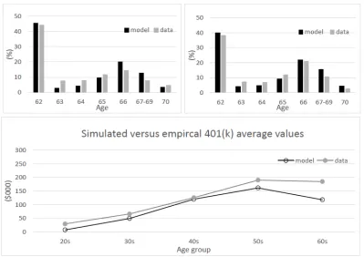
Figure 1 (top) presents claiming rates generated by our life-cycle model (dark bars) versus empirical claiming rates (light bars) reported by the U.S. Social Security Administration for the year 2015 for nondisabled men and women. Here we see that our
model closely tracks the empirically-observed early claiming age peak at age 62, as well as the second peak at the Full Retirement Age (66). The lower panel of Figure 1
Figure 1: Social Security Claiming Patterns for Women and Men, and 401(k) Asset Values (model versus data)
Notes: The top two panels compare claiming rates generated by our life-cycle models and empirical claiming rates reported by the US Social Security Administration for the year 2015 (excluding disability). Expected values are calculated from 100,000 simulated life cycles based on optimal feedback controls. Results for the entire female (male) population are computed using income profile for three education levels: 61% Coll+; 28% HS; 11% <HS (57% Coll+; 30% HS; 13%<HS). Parameters used for the baseline calibration are as follows: risk aversion ρ=5; time preference β=0.96; leisure preference α = 1.2; endogenous retirement ages 62 to 70. Social Security benefits are
What would Rothification do?
We next illustrate how switching from traditional EET to a TEE tax regime for retirement savings would affect claiming ages, assets held inside and outside tax-qualified retirement plans, consumption, hours of work, asset and consumption inequality, and tax payments over the life cycle. In addition, we study how the results would differ, if the very low interest rate environment of the last decade (𝑓𝑓= 1%) were to be replaced by a more historically “normal” return regime (𝑓𝑓= 3%).
Asset accumulation patterns
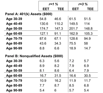
Table 1 offers an accounting of how the tax regime change alters asset allocation patterns in the 401(k) accounts versus nontax-qualified assets. Here we focus on life-cycle asset accumulation patterns under the EET/TEE regimes, as well as the low/high expected return scenarios. Most strikingly, we see that assets in 401(k) plans (Panel A) are lower under the Rothification regime, particularly in later life, compared to the higher levels under the EET regime. This shortfall is greater in the higher return regime, such that tax qualified assets are always larger in the EET environment. By contrast,
Table 1: Life-cycle Asset Accumulation Patterns under EET versus TEE Tax Regimes, and Low versus High Expected Return Scenarios
r=1 % r=3 %
EET TEE EET TEE
Panel A: 401(k) Assets ($000)
Age 30-39 54.8 46.6 61.5 51.5
Age 40-49 130.6 110.2 149.5 114 Age 50-59 174.7 147.3 201.7 148.8 Age 60-69 127.1 91.1 162.9 105.3
Age 70-79 87.6 67.1 128.6 94.9
Age 80-89 43.6 34.3 75.5 58
Age 90-99 8.8 6.6 18.9 14.7
Panel B: Nonqualified Assets ($000)
Age 30-39 6.3 5.6 7.2 5.7
Age 40-49 8.9 8.2 7.9 6.9
Age 50-59 8.1 8.6 6.4 7.9
Age 60-69 16.7 31.5 16.6 30.5
Age 70-79 10.9 16.2 11.9 11.7
Age 80-89 7.7 8.7 8.5 6.8
Age 90-99 5.4 6 5.7 5.4
Notes: The two panels show expected assets by age in tax-qualified 401(k) plans and nonqualified assets for low- and high-interest rate (1% and 3%), and different tax regimes. Expected values are based on 100,000 simulated life cycles using optimal feedback controls from the life-cycle model. The assumed risk premium for stock returns is 5% and return volatility 18%. For other parameters, see Figure 1. Source: Authors’ calculations.
Impacts on consumption and work hours
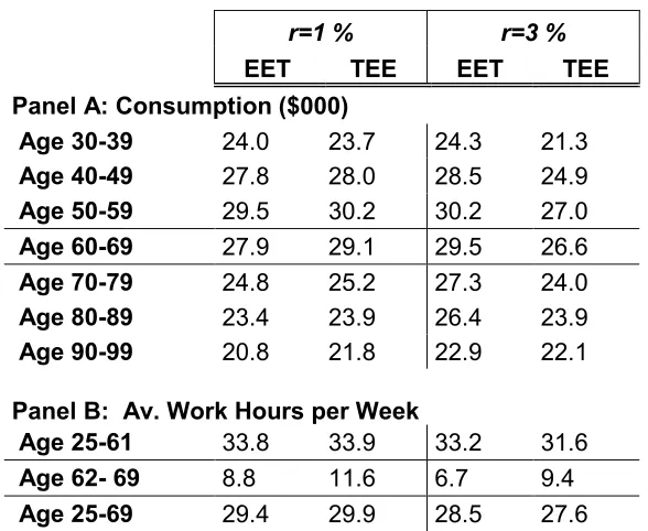
Table 2 evaluates the effects of moving from an EET to a TEE regime on
the real return were instead 𝑓𝑓= 3%, average consumption under TEE would be lower for all age groups, compared to the EET case. In addition, during the work life, work effort would be about two hours per week lower under TEE. Nevertheless, in the Social Security benefit claiming window, people work about three hours more per week under the TEE regime. Overall, Rothification reduces work over the lifetime but pushes out retirement claiming, compared to the EET tax environment.
Table 2: Life-Cycle Consumption and Working Hours under EET versus TEE Tax Regimes, and Low versus High Expected Return Scenarios
r=1 % r=3 %
EET TEE EET TEE
Panel A: Consumption ($000)
Age 30-39 24.0 23.7 24.3 21.3 Age 40-49 27.8 28.0 28.5 24.9 Age 50-59 29.5 30.2 30.2 27.0 Age 60-69 27.9 29.1 29.5 26.6 Age 70-79 24.8 25.2 27.3 24.0 Age 80-89 23.4 23.9 26.4 23.9 Age 90-99 20.8 21.8 22.9 22.1 Panel B: Av. Work Hours per Week
Age 25-61 33.8 33.9 33.2 31.6 Age 62- 69 8.8 11.6 6.7 9.4 Age 25-69 29.4 29.9 28.5 27.6
Notes: The two panels report average consumption and weekly work hours for low and high r
Impact on claiming ages
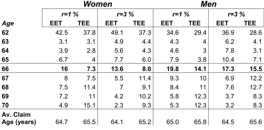
Table 3 shows how Social Security benefit claiming ages would change by sex across tax regimes and under the low- versus high-interest rate scenarios. In both tax regimes, men’s and women’s average retirement ages are later when interest rates are low (𝑓𝑓= 1%). This is because delaying Social Security is similar to buying a deferred annuity.13 Therefore, it is more attractive to draw down one’s 401(k) account to delay Social Security claiming, compared to keeping the money in the retirement account and earning (uncertain) investment returns.
Overall, the TEE regime’s lower marginal tax rate on 401(k) payouts induces workers to defer Social Security claiming more than under the EET regime. This may be explained as follows: Some workers with sufficient retirement plan assets want to retire, but they find it attractive to wait to claim Social Security so as to boost those benefits via the delayed claiming factors (6% to 8% increase per year of delayed claiming).
Meanwhile, financing consumption during this no-work phase requires them to withdraw from their 401(k) assets. Under an EET regime, workers must pay income taxes on their pension withdrawals. Thus, the attraction of earning higher Social Security benefits by delaying claiming must be weighed against the disadvantage of paying high income taxes on withdrawals. If the tax burden on withdrawals is heavier than the advantage of receiving higher Social Security benefits, it is rational to claim earlier. This tradeoff must also take into account the fact that only a portion of Social Security benefits are included in taxable income (up to 50% could be tax-free). Accordingly, the net-of-tax gain from
delaying Social Security claiming is relatively small in the EET scenario. The effect is stronger when interest rates are high, because workers build more assets in their 401(k) accounts.
Table 3: Social Security Claiming Patterns (in %) for Women and Men under EET versus TEE Tax Regimes, and Low versus High Expected Return Scenarios
Notes: We report the average claiming age for low and high r (1% and 3%) by sex, for the two different tax regimes (EET versus TEE) derived from 100,000 simulated life cycles based on optimal feedback controls from the life-cycle model. The assumed risk premium for stock returns is 5% and return volatility 18%. For other parameters, see Figure 1. Source: Authors’
calculations.
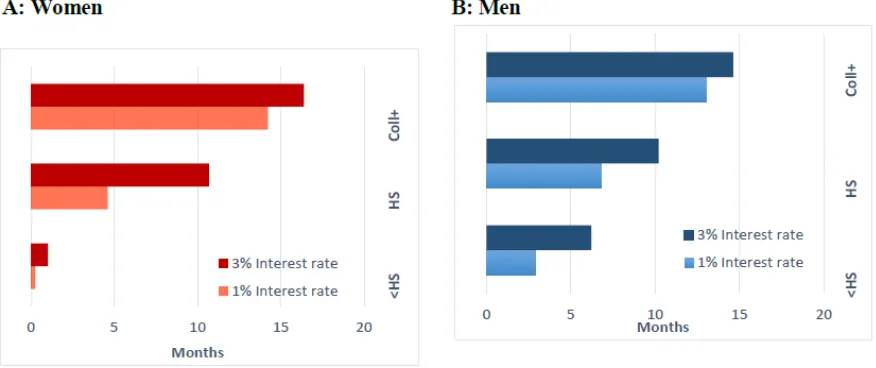
The average claiming-age changes do obscure some interesting differences across population subgroups, as can be seen in Figure 2. Specifically, claiming
behavior of the least-educated high school dropouts is relatively similar in the EET and TEE regimes, primarily because this group saves and accumulates fewer assets than the better-educated. Moreover, the changes in claiming ages for this group are small under both interest rate environments. For example, women (men) without a high
school degree work only 0.5 (3) month more under the TEE regime in a low-interest rate
Women
Men
r=1 % r=3 % r=1 % r=3 %
Age EET TEE EET TEE EET TEE EET TEE
62 42.5 37.8 49.1 37.3 34.6 29.4 36.9 28.6
63 3.1 3.1 4.9 4.4 4.3 4 6.2 4.1
64 3.9 2.8 5.6 4.3 4.6 3 7.8 3.1
65 6.7 4 7.7 6.0 7.9 3.8 10.4 7.1
66 16 7.3 13.6 8.0 19.8 14.1 17.3 15.5
67 8 7.5 5.5 11.4 9.3 10 6.9 12.2
68 7.5 11.4 7 9.1 8.4 11 7.6 12.7
69 7.2 11 4.2 10.2 5.8 12.3 3.7 8.3
70 4.9 15.1 2.3 9.3 5.3 12.3 3.2 8.3
Av. Claim
environment, while Coll+ men and women defer claiming benefits by more than a year under both interest rate environments. The impact is strongest for college-educated women who work 16 months longer given a high real rate in the TEE versus EET setup. Accordingly, more educated and wealthier workers are predicted to work substantially longer under Rothification, with a much smaller impact on the less-educated.
Figure 2: Average Claiming Age Differences by Education: TEE (Roth) versus EET Tax Regimes, and Low- versus High-Return Scenarios
Notes: We report the average claiming age difference for EET versus TEE for r=1% and 3% by sex and education groups <HS, HS, Coll+, derived from 100,000 simulated life cycles based on optimal feedback controls from the life-cycle model. Preference parameters are as follows: risk aversion ρ=5; time preference β=0.96; leisure preference α = 1.2. The endogenous retirement age is between ages 62 to 70.The assumed risk premium for stock returns is 5% and return volatility 18%. Tax bracket are based on 2018 regulations (as described in Appendix B). Source: Authors’ calculations.
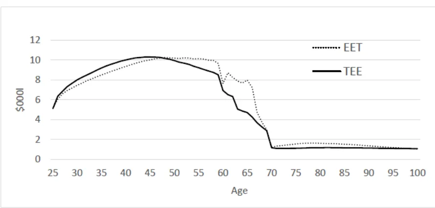
Impacts on tax payments over the life cycle
and penalty taxes for early withdrawals for the overall population comprised by our six subgroups. Both scenarios assume a low and persistent interest rate of 1%. As
anticipated, tax payments under EET are lower during the first 25 years of the worklife, since 401(k) contributions are not part of taxable income; by contrast, under the TEE regime, workers must pay taxes on both own and employer matching contributions. Yet the situation changes around age 50 when tax payments rise in the EET regime, and the difference is particularly marked between ages 62 and 70. Thereafter, tax payments in both the EET and TEE scenarios are relatively low.
The explanation is that, in both tax regimes, workers begin curtailing their work hours after age 50 and finance their consumption by 401(k) withdrawals. From age 60 onward, 401(k) withdrawals are not subject to the 10% penalty tax in both tax regimes, but withdrawals from EET accounts are part of taxable income which results in higher tax payments — in contrast to the TEE world. The difference in tax payment is
Figure 3: Average Annual Tax Payments per Individual: EET versus TEE (Roth) Tax Regimes
Notes: The figure shows average annual tax payments (sum of income taxes, payroll taxes, and penalty tax for early withdrawals) over the life cycle per individual for EET versus TEE taxation based on low interest rates (1%). Values are based on 100,000 simulated life cycles for each of the six subgroups (men/women and three education groups) using optimal feedback controls from the life-cycle model. Results for the entire population are computed using the following weights for the three education levels: women (61% Coll+; 28% HS; 11% <HS) and men (57% Coll+; 30% HS; 13%<HS); the weights for women is 51% and for men 49%. Further notes on parameters see Figure 2.
tax payments average 6% ($24,000) more in the EET world when the interest rate is low; the difference increases to about 10% ($42,000) if the real rate is 3%. Overall, we conclude that tax payments are higher in the short run in the TEE regime, but lower in the long run.
Table 4: Sum of Average Lifetime Tax Payments per Individual: EET versus TEE (Roth) Tax Regimes, and Low versus High Expected Return Scenarios
r = 1 % r = 3 %
EET TEE EET TEE
Age 25-49 214.6 225.4 213.9 222.7 Age 50-69 167.4 141.2 165.8 133.4 Age 70-100 43.4 35.2 54.5 36.3 Age 25-100 425.4 401.8 434.2 392.4
Notes: The table reports average lifetime tax payments (sum of income taxes, payroll taxes, and penalty tax for early withdrawals) per individual for EET versus TEE taxation and for low and high interest rates (1% and 3%). Values are based on 100,000 simulated life cycles for each of the six subgroups (men/ women and three education groups) using optimal feedback controls from the life-cycle model. Results for the entire population are computed using the following weights for the three education levels: women (61% Coll+; 28% HS; 11% <HS) and men (57% Coll+; 30% HS; 13%<HS); the weights for women is 51% and for men, 49%. For further notes on parameters see Figure 2.
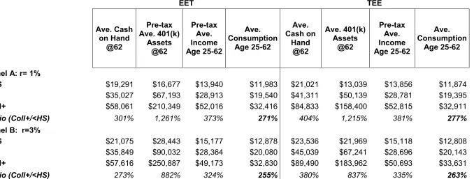
Impact on Inequality
Table 5: Asset and Consumption Inequality by Education under EET versus TEE Tax Regimes, and Low versus High Expected Return Scenarios
EET TEE
Ave. Cash on Hand
@62 Pre-tax Ave. 401(k) Assets @62 Pre-tax Ave. Income Age 25-62 Ave. Consumption Age 25-62 Ave. Cash on Hand @62 Ave. 401(k) Assets @62 Pre-tax Ave. Income Age 25-62 Ave. Consumption Age 25-62
Panel A: r= 1%
<HS $19,291 $16,677 $13,940 $11,983 $21,021 $13,039 $13,856 $11,874
HS $35,027 $67,193 $28,913 $19,540 $41,311 $50,139 $28,781 $19,395
Coll+ $58,061 $210,349 $52,016 $32,416 $84,833 $158,400 $52,815 $32,911
Ratio (Coll+/<HS) 301% 1,261% 373% 271% 404% 1,215% 381% 277%
Panel B: r=3%
<HS $21,075 $28,443 $15,177 $12,878 $23,536 $21,969 $15,118 $12,808
HS $35,849 $90,032 $28,364 $20,080 $45,039 $67,241 $28,696 $20,143
Coll+ $57,616 $250,887 $49,173 $32,830 $89,490 $183,962 $50,693 $33,631
Following Lusardi, Michaud, and Mitchell (2017), we measure relative wealth, income, and consumption inequality in terms of the ratio of college graduates to high school dropouts as of age 62. The higher is this ratio, the greater the inequality along this dimension. Regardless of the interest rate environment, we see that inequality measured in this way is greater under the TEE regime for all four metrics. For
example, under the EET regime, for 𝑓𝑓= 1%, workers with Coll+ education have three times the assets in nonqualified accounts compared to high school dropouts; this rises to four times under the TEE regime. Due to the different tax regimes, income inequality also rises by 8 percentage points under the TEE regime when interest rates are low, and by 11 percentage points for the higher interest rate. Absolute asset levels in 401(k) accounts are not directly comparable across the two tax regimes, but the inequality measure is comparable and it is 6 percentage points higher in the TEE case. Finally, consumption inequality is greater under TEE taxation of retirement savings.
Conclusions
This paper evaluates whether adopting a different tax treatment of retirement plan contributions would materially change Social Security benefit claiming ages and work hours, consumption, and asset allocation of workers looking ahead to
retirement. We also assess whether the lower-paid would behave differently from the higher-paid, in terms of change in claiming, saving inside and outside the Roth
higher benefits for low-wage workers than for the higher paid. Given these realities, an EET scheme enhances the progressivity of overall old-age income (pension account withdrawals plus Social Security benefits), whereas a TEE structure treats pension benefits more neutrally. Accordingly, it is theoretically impossible to predict how Rothification will alter household behavior without taking into account the rich institutional details confronting real-world consumers, along with the economic environment, capital and labor market risk, and uncertain lifetimes.
References
Arias, E. (2010). United States Life Tables, 2005. National Vital Statistics Reports
58(10).
U.S. National Center for Health Statistics: Hyattsville, Maryland.
Brown, Jeffrey R. 2001. Private Pensions, Mortality Risk, and the Decision to Annuitize. Journal of Public Economics 82(1): 29-62.
Carroll, C. D. and A. A. Samwick. (1997). The Nature of Precautionary Wealth. Journal of Monetary Economics. 40(1): 41-71.
Chai, J., W. Horneff, R. Maurer, and O. S. Mitchell. (2011). Optimal Portfolio Choice over the Life Cycle with Flexible Work, Endogenous Retirement, and Lifetime Payouts. Review of Finance. 15(4): 875-907.
Cocco, J., F. Gomes, and P. Maenhout. (2005). Consumption and Portfolio Choice over the Life Cycle. Review of Financial Studies. 18(2): 491-533.
Employee Benefit Research Institute. 2017. What Does Consistent Participation in 401(k) Plans Generate? Changes in 401(k) Plan Account Balances, 2010– 2015. EBRI Issue BRIEF No.439, Oct. 2017
Gomes, F. J., L. J. Kotlikoff, and L. M. Viceira. (2008). Optimal Life-Cycle Investing with Flexible Labor Supply: A Welfare Analysis of Life-Cycle Funds. American
Economic Review: Papers & Proceedings. 98(2): 297-303.
Gomes, F. J., and A. Michaelides. 2005. Optimal Life-Cycle Asset Allocation: Understanding the Empirical Evidence. The Journal of Finance. 60(2):869-904.
Gomes, F., A. Michaelides, and V. Polkovnichenko (2009). Optimal Savings with Taxable and Tax-Deferred Accounts. Review of Economic Dynamics. 12(4): 718-735.
Hallez, E. (2017). How a GOP Roth Plan Could Impact Retirement Savings.
https://www.ignites.com/c/1781243/209413?referrer_module=SearchSubFrom IG&highlight=How%20a%20GOP%20Roth%20Plan%20Could%20Impact%20 Retirement%20Savings
Horneff, V., R. Maurer, and O.S. Mitchell. (2018). How Low Returns Alter Optimal Life Cycle Saving, Investment, and Retirement Behavior. In R. Clark, R. Maurer, and O. S. Mitchell, eds. How Persistent Low Returns Will Shape Saving and
Retirement. (2018). Oxford: Oxford University Press. 119-131.
Horneff, V., R. Maurer, and O.S. Mitchell. (2019). How Will Persistent Low Expected Returns Shape Household Economic Behavior? Journal of Pension
Economics and Finance 18, 612-622.
Horneff, V., R. Maurer, O.S. Mitchell, and R. Rogalla. (2015). Optimal Life Cycle Portfolio Choice with Variable Annuities Offering Liquidity and Investment Downside Protection. Insurance: Mathematics and Economics. 63(1): 91-107.
Horneff, V., R. Maurer, and O.S. Mitchell. (2016). Putting the Pension Back in 401(k) Plans: Optimal versus Default Longevity Income Annuities. NBER Working Paper 22717
Hubener, A., R. Maurer, and O. S. Mitchell. (2016). How Family Status and Social Security Claiming Options Shape Optimal Life Cycle Portfolios. Review of Financial Studies. 29(4): 937-978.
Internal Revenue Service (IRS 2015a). Form 1040 (Tax Tables): Federal Tax Rates,
Personal Exemptions, and Standard Deductions. Downloaded 09/13/2018.
https://www.irs.com/articles/2015-federal-tax-rates-personal-exemptions-and-standard-deductions
Internal Revenue Service (IRS 2015b). Retirement Plan and IRA Required minimum
distributions FAQs. https://www.irs.gov/pub/irs-prior/p590b--2015.pdf
Internal Revenue Service (IRS 2018). Form 1040 (Tax Tables): Federal Tax Rates,
Personal Exemptions, and Standard Deductions. Downloaded 08/26/2019.
Love, D.A. (2007). What Can Life-Cycle Models Tell U.S. about 401(k) Contributions and Participation? Journal of Pension Economics and Finance. 6(2): 147-185.
Love, D.A. (2010). The Effects of Marital Status and Children on Savings and Portfolio Choice. Review of Financial Studies. 23(1): 385-432.
Lusardi, A.M., P.C. Michaud, and O.S. Mitchell (2017). “Optimal Financial Literacy and Wealth Inequality.” Journal of Political Economy. 125(2): 431-477.
Maurer, R., O.S. Mitchell, R. Rogalla, and T. Schimetschek (2017). Optimal Social Security Claing Behavior Under Lump Sum Incentives: Theory and Evidence. NBER Working Paper 23073.
National Center on Education Statistics. (2016). Digest of Education Statistics 52nd Edition, Table 104.30. https://nces.ed.gov/pubs2017/2017094.pdf (download 09.13.2018).
Schoeff, M. (2017). Promises by Congress to Protect Retirement-savings Incentives Don't Ease Advocates. Jul 12. InvestmentNews.com.
https://www.investmentnews.com/article/20170712/FREE/170719976/promise s-by-congress-to-protect-retirement-savings-incentives-dont
Shoven, J.B., and S. N. Slavov. (2014). Does it Pay to Delay Social Security? Journal
of Pension Economics and Finance. 13 (2): 121-144.
Shoven, J.B., and S. N. Slavov. (2012). The Decision to Delay Social Security Benefits: Theory and Evidence. NBER Working Paper 17866.
Sibaie, A. (2017). What Rothification Means for Tax Reform. The Tax Foundation. Washington, D.C. https://taxfoundation.org/what-rothification-means-for-tax-reform/
Statman, M. (2017). Critically, 'Rothification' of 401(k)’s not Harmful to Lower Incomes. TheHill.com.
Thornton, Nick. (2017). Asset Managers’ Profits Threatened by Rothification. benefitspro.com, September. http://www.benefitspro.com/2017/09/07/asset-managers-profits-threatened-by-rothification?t=retirement&slreturn=1508873159&page=3&page_all=1
U.S. Department of Labor (US DOL). (2016). Economic News Release Table A-4. Employment Status of the Civilian Population 25 Years and Over by
Educational Attainment. Washington, DC.
U.S. Department of Labor (US DOL). (2006). Fact Sheet: Default Investment
Alternatives under Participant-Directed Individual Account Plans. Washington, DC.
https://www.dol.gov/ebsa/newsroom/fsdefaultoptionproposalrevision.html
U.S. Department of Labor (US DOL). (nd). Fact Sheet: Regulation Relating to Qualified Default Investment Alternatives in Participant-Directed Individual
Account Plans. Washington, DC.
https://www.dol.gov/ebsa/newsroom/fsqdia.html
U.S. Social Security Administration (US SSA). (nd_a).Primary Insurance Amount.
Washington, DC. https://www.ssa.gov/oact/cola/bendpoints.html
U.S. Social Security Administration (US SSA). (nd_b). Fact Sheet:Benefit Formula Bend Points. Washington, DC. https://www.ssa.gov/oact/cola/piaformula.html
U.S. Social Security Administration (US SSA). (nd_c). Incentivizing Delayed Claiming of Social Security Retirement Benefits Before Reaching the Full
Retirement Age. Washington, DC.
https://www.ssa.gov/policy/docs/ssb/v74n4/v74n4p21.html
U.S. Social Security Administration (US SSA). (nd_d).Benefits Planner: Income Taxes and Your Social Security Benefit.Washington, DC.
https://www.ssa.gov/planners/taxes.html
U.S. Social Security Administration. (2014). Annual Statistical Supplement to the
Social Security Bulletin. Washington, DC.
U.S. Social Security Administration. (2015). Annual Statistical Supplement to the
Social Security Bulletin, 2015 (Table 6.B5). Washington, DC.
Willson, Nicolle (2019). Safe Harbor 401(k): The 2019 Guide for Business Owners.
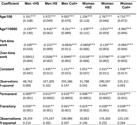
Appendix A: Wage rate estimation
We calibrated the wage rate process using the Panel Study of Income Dynamics (PSID) 1975 to 2015, from ages 25 to 69. During the work life, each individual’s labor income profile has deterministic, permanent, and transitory components with uncorrelated and normally distributed shocks according to
𝑙𝑙𝑝𝑝(𝑁𝑁𝑡𝑡) ~𝑁𝑁(−0.5𝜎𝜎𝑛𝑛2, 𝜎𝜎𝑛𝑛2) and 𝑙𝑙𝑝𝑝(𝑈𝑈𝑡𝑡) ~𝑁𝑁(−0.5𝜎𝜎𝑢𝑢2, 𝜎𝜎𝑢𝑢2). The wage rate values are
expressed in $2015. These are estimated separately by sex and by educational level. The educational groupings are: less than high school (<HS), high school graduate (HS), and those with at least some college (Coll+). Extreme observations below $5 per hour and above the 99th percentile are dropped.
We use a second order polynomial in age and dummies for employment status. The regression function is:
ln (𝑤𝑤𝑖𝑖,𝑦𝑦) =𝛽𝛽1∗ 𝑇𝑇𝑎𝑎𝑝𝑝𝑖𝑖,𝑦𝑦 +𝛽𝛽2∗ 𝑇𝑇𝑎𝑎𝑝𝑝𝑖𝑖2,𝑦𝑦+ 𝛽𝛽5∗ 𝐸𝐸𝑆𝑆𝑖𝑖,𝑦𝑦+𝛽𝛽𝑤𝑤𝑡𝑡𝑤𝑤𝑤𝑤𝑠𝑠∗ 𝑤𝑤𝑇𝑇𝑤𝑤𝑝𝑝𝑑𝑑𝑢𝑢𝑚𝑚𝑚𝑚𝑑𝑑𝑝𝑝𝑑𝑑, (A1)
where log (𝑤𝑤𝑖𝑖,𝑦𝑦) is the natural log of wage at time y for individual i, age is the age of
the individual divided by 100, ES is the individual’s employment status, and wave dummies control for year-specific shocks. For employment status, we include three groups depending on work hours per week as follows: part-time worker (≤ 20 hours), full-time worker (< 20 & ≤ 40 hours) and overtime worker (< 40 hours). OLS
𝑓𝑓𝑖𝑖,𝑑𝑑 =∑𝑑𝑑−1𝑠𝑠=0(𝑁𝑁𝑡𝑡+𝑠𝑠) +𝑈𝑈𝑖𝑖,𝑡𝑡+𝑑𝑑 − 𝑈𝑈𝑖𝑖,𝑡𝑡. (A2)
We then regress the 𝑤𝑤𝑖𝑖𝑑𝑑 =𝑓𝑓�����𝚤𝚤2,𝑑𝑑 on the lengths of time d between waves and a
constant:
𝑤𝑤𝑖𝑖𝑑𝑑 =𝛽𝛽1⋅ 𝑑𝑑+𝛽𝛽2⋅2 +𝑝𝑝𝑖𝑖𝑑𝑑, (A3)
where the variance of the permanent factor 𝜎𝜎𝑁𝑁2 =𝛽𝛽1 and the 𝜎𝜎𝑈𝑈2 = 𝛽𝛽2 represents the
Table A1: Regression results for wage rates Coefficient Men <HS Men HS Men Coll+ Women
<HS Women HS Women Coll+
Age/100 3.161*** 5.972*** 9.092*** 1.256*** 2.767*** 4.731***
(0.108) (0.049) (0.070) (0.110) (0.046) (0.072)
Age²/10000 -3.329*** -6.416*** -9.351*** -1.339*** -2.915*** -4.960***
(0.130) (0.062) (0.089) (0.131) (0.059) (0.094)
Part-time
work -0.109*** -0.153*** -0.0826*** -0.0858*** -0.129*** -0.0847***
(0.020) (0.009) (0.011) (0.006) (0.003) (0.004)
Over-time
work 0.00412 0.0506*** 0.0949*** 0.0158*** 0.0748*** 0.106***
(0.004) (0.002) (0.002) (0.006) (0.002) (0.003)
Constant 1.807*** 1.435*** 1.151*** 2.051*** 2.015*** 1.938***
(0.042) (0.012) (0.015) (0.037) (0.011) (0.017)
Observations 48,762 327,305 293,386 31,788 290,597 225,211
R-squared 0.069 0.102 0.147 0.032 0.044 0.092
Permanent 0.009*** 0.013*** 0.019*** 0.008*** 0.013*** 0.019***
(0.001) (0.0002) (0.0003) (0.0001) (0.0002) (0.001)
Transitory 0.028*** 0.031** 0.041*** 0.023*** 0.028*** 0.038***
(0.001) (0.001) (0.001) (0.002) (0.001) (0.001)
Observations 28,359 175,247 140,984 20,863 176,304 123,145
R-squared 0.214 0.283 0.307 0.146 0.255 0.264
Appendix B: Modeling retirement accounts
We embed a U.S.-type progressive tax system in our model to explore the impact of having access to a qualified (tax-sheltered) pension account of the EET versus the TEE (Roth) type.14 (All values are in $2015 and relevant amounts are
inflation adjusted yearly). Here the worker must pay taxes on labor income and on capital gains from investments in bonds and stocks. During the working life, he invests 𝐴𝐴𝑡𝑡in a tax-qualified pension account which reduces his taxable income;
contributions can be made to an annual maximum amount 𝐷𝐷𝑡𝑡=$18,000 (and from age
50 an additional $6,000 catch up is feasible). Correspondingly, withdrawals 𝑊𝑊𝑡𝑡 from
the tax-qualified account increase taxable income. Finally, the worker’s taxable income is reduced by a general standardized deduction 𝐺𝐺𝐷𝐷. For a single person, this deduction was in 2015 $6,300 (in 2018 $12,000) per year. Consequently, taxable income during the working age is given by:
EET 𝑌𝑌𝑡𝑡+1𝑡𝑡𝑡𝑡𝑡𝑡 = max�max�𝑆𝑆𝑡𝑡⋅(𝑅𝑅𝑡𝑡+1−1) +𝐵𝐵𝑡𝑡⋅ �𝑅𝑅𝑓𝑓−1�; 0�+
𝑌𝑌𝑡𝑡+1(1− ℎ𝑡𝑡) +𝑊𝑊𝑡𝑡−min(𝐴𝐴𝑡𝑡;𝐷𝐷𝑡𝑡+𝑐𝑐𝑇𝑇𝑡𝑡𝑐𝑐ℎ𝑢𝑢𝑝𝑝)− 𝐺𝐺𝐷𝐷; 0�, and
(B1) TEE 𝑌𝑌𝑡𝑡+1𝑡𝑡𝑡𝑡𝑡𝑡 = max�max�𝑆𝑆
𝑡𝑡⋅(𝑅𝑅𝑡𝑡+1−1) +𝐵𝐵𝑡𝑡⋅ �𝑅𝑅𝑓𝑓−1�; 0�+𝑀𝑀𝑡𝑡+
𝑌𝑌𝑡𝑡+1(1− ℎ𝑡𝑡)− 𝐺𝐺𝐷𝐷; 0�.
For Social Security (𝑌𝑌𝑡𝑡+1) taxation, we use the following rules: when the retiree’s
combined income15 is between $25,000 and $34,000 (more than $34,000), 50%
(85%) of benefits are taxed. After retirement, we set 𝐴𝐴𝑡𝑡= 0, i.e. no further
contributions in 401(k) retirement plans are possible.
14 That is, contributions and investment earnings in the account are tax exempt (E), while payouts are taxed (T).
15Combined income issum of adjusted gross income, nontaxable interest, and half of his
In line with U.S. rules for federal income taxes, our progressive tax system has seven income tax brackets (IRS 2015a). These brackets 𝑑𝑑 = 1, … ,7 are defined by a lower and an upper bound of taxable income 𝑌𝑌𝑡𝑡+1𝑡𝑡𝑡𝑡𝑡𝑡 ∈[𝑙𝑙𝑏𝑏𝑖𝑖,𝑢𝑢𝑏𝑏𝑖𝑖] and determine a
marginal tax rate 𝑓𝑓𝑖𝑖𝑡𝑡𝑡𝑡𝑡𝑡. In 2018, the marginal taxes rates for a single household were
10% from $0 to $9,225, 12% from $9,225 to $38,700, 22% from $38,701 to $82,500, 24% from $82,501 to $157,500, 32% from $157,500 to $200,000, 35% from
$200,001 to $500,000 and 37% greater than $500,000 (see IRS 2018). Based on these tax brackets, the dollar amount of taxes payable is given by:16
𝐼𝐼𝑇𝑇𝑡𝑡+1𝑡𝑡𝑡𝑡𝑡𝑡 =(𝑌𝑌𝑡𝑡𝑡𝑡𝑇𝑇𝑥𝑥+1− 𝑙𝑙𝑏𝑏7)⋅1�𝑌𝑌𝑡𝑡𝑡𝑡𝑇𝑇𝑥𝑥+1≥𝑙𝑙𝑏𝑏7�⋅ 𝑓𝑓7
𝑡𝑡𝑇𝑇𝑥𝑥
+�(𝑌𝑌𝑡𝑡𝑡𝑡𝑇𝑇𝑥𝑥+1− 𝑙𝑙𝑏𝑏
6)⋅1�𝑙𝑙𝑏𝑏7>𝑌𝑌𝑡𝑡𝑇𝑇𝑥𝑥𝑡𝑡+1≥𝑙𝑙𝑏𝑏7�+(𝑢𝑢𝑏𝑏6− 𝑙𝑙𝑏𝑏6)⋅1�𝑌𝑌𝑡𝑡𝑡𝑡𝑇𝑇𝑥𝑥+1≥𝑙𝑙𝑏𝑏7��⋅ 𝑓𝑓6𝑡𝑡𝑇𝑇𝑥𝑥
+�(𝑌𝑌𝑡𝑡𝑡𝑡𝑇𝑇𝑥𝑥+1− 𝑙𝑙𝑏𝑏5)⋅1�𝑙𝑙𝑏𝑏6>𝑌𝑌𝑡𝑡𝑡𝑡𝑇𝑇𝑥𝑥+1≥𝑙𝑙𝑏𝑏5�+(𝑢𝑢𝑏𝑏5− 𝑙𝑙𝑏𝑏5)⋅1�𝑌𝑌𝑡𝑡𝑡𝑡𝑇𝑇𝑥𝑥+1≥𝑙𝑙𝑏𝑏6��⋅ 𝑓𝑓5
𝑡𝑡𝑇𝑇𝑥𝑥
+�(𝑌𝑌𝑡𝑡𝑡𝑡𝑇𝑇𝑥𝑥+1− 𝑙𝑙𝑏𝑏4)⋅1�𝑙𝑙𝑏𝑏5>𝑌𝑌𝑡𝑡𝑡𝑡𝑇𝑇𝑥𝑥+1≥𝑙𝑙𝑏𝑏4�+(𝑢𝑢𝑏𝑏4− 𝑙𝑙𝑏𝑏4)⋅1�𝑌𝑌𝑡𝑡𝑡𝑡𝑇𝑇𝑥𝑥+1≥𝑙𝑙𝑏𝑏5��⋅ 𝑓𝑓4
𝑡𝑡𝑇𝑇𝑥𝑥
+�(𝑌𝑌𝑡𝑡𝑡𝑡𝑇𝑇𝑥𝑥+1− 𝑙𝑙𝑏𝑏3)⋅1�𝑙𝑙𝑏𝑏4>𝑌𝑌𝑡𝑡𝑡𝑡𝑇𝑇𝑥𝑥+1≥𝑙𝑙𝑏𝑏3�+(𝑢𝑢𝑏𝑏3− 𝑙𝑙𝑏𝑏3)⋅1�𝑌𝑌𝑡𝑡𝑇𝑇𝑥𝑥𝑡𝑡+1≥𝑙𝑙𝑏𝑏4��⋅ 𝑓𝑓3𝑡𝑡𝑇𝑇𝑥𝑥
+�(𝑌𝑌𝑡𝑡𝑡𝑡𝑇𝑇𝑥𝑥+1− 𝑙𝑙𝑏𝑏2)⋅1�𝑙𝑙𝑏𝑏3>𝑌𝑌𝑡𝑡𝑡𝑡𝑇𝑇𝑥𝑥+1≥𝑙𝑙𝑏𝑏2�+(𝑢𝑢𝑏𝑏2− 𝑙𝑙𝑏𝑏2)⋅1�𝑌𝑌𝑡𝑡𝑇𝑇𝑥𝑥𝑡𝑡+1≥𝑙𝑙𝑏𝑏3��⋅ 𝑓𝑓2𝑡𝑡𝑇𝑇𝑥𝑥
+�(𝑌𝑌𝑡𝑡𝑡𝑡𝑇𝑇𝑥𝑥+1− 𝑙𝑙𝑏𝑏1)⋅1�𝑙𝑙𝑏𝑏2>𝑌𝑌𝑡𝑡𝑡𝑡𝑇𝑇𝑥𝑥+1≥𝑙𝑙𝑏𝑏1�+(𝑢𝑢𝑏𝑏1− 𝑙𝑙𝑏𝑏1)⋅1�𝑌𝑌𝑡𝑡𝑡𝑡𝑇𝑇𝑥𝑥+1≥𝑙𝑙𝑏𝑏2��⋅ 𝑓𝑓1
𝑡𝑡𝑇𝑇𝑥𝑥
(B2)
where, for 𝐴𝐴 ⊆ 𝑋𝑋, the indicator function 1𝐴𝐴 →{0, 1} is defined as:
1𝐴𝐴(𝑥𝑥) =�
1 | 𝑥𝑥 ∈ 𝐴𝐴
0 | 𝑥𝑥 ∉ 𝐴𝐴 . (B3)