The use of admissions simulation to stabilize ancillary workloads

The

use

of

admissions simulation

to

stabilize

ancillary

workloads

Walton M. Hancock

Department

of Industrial and

Operations Engineering

University

of

Michigan

IOE

Building,

1205 Beal Avenue Ann

Arbor,

Michigan

48109

Paul F. Walter Walter Software

Engineering

3692 Valentine Road

Whitmore

Lake,

Michigan

48189

WALTON M. HANCOCK is Professor of Industrial and Operations

Engineering

and Professor of

Hospital

Administration at The Univer-sity

of Michigan.

His main area of interest is the use of

computer-aided

systems to reduce the costs of _operating

hospitals.

His most recent

major

publications

are The &dquo;ASCS’; The _Inpatient Admissions

Scheduling

and Control System, and Advanced Work Measurement. He has three

degrees,

including

a Doctor of

Engineering

from The Johns

Hopkins

University.

PAUL F. WALTER received his BSE from The University of

Michigan

College

of _Engineering in

applied

mathematics in 1973.

Following

a

year of software

development

for process control systems at Ann

Ar-bor Computer Corporation, he

joined

the staff of The _Department of

Hospital

Administration in the School of Public Health at The University of

Michigan.

There he

participated

in the research and

development

of an admission

scheduling

and control system, a nurse

staffing

_system,

and other _management information _systems for

hospitals.

In 1982 he left the _University but continued his efforts in the

development

and

implementation

of

hospital

cost containment systems as the owner

of Walter Software _Engineering. Mr. Walter is the coauthor of four

published

papers, more than a dozen _reports and the book The &dquo;ASCS&dquo;

Inpatient

Scheduling

and Control System.

ABSTRACT

As _part of the

planning

of a new

hospital,

an

analysis

was

per-formed to determine the number of

procedures

that would be

performed

in each of nineteen

ancillary departments

on a

day

of the week basis. Because the

planned

occupancy was not the maximum

possible,

_attempts were made

using

simulation to smooth the

daily ancillary

loads

by

varying

the admission

day

of

elective,

urgent

inpatient

and

outpatient

loads. The

methodology,

sample

outputs, and main conclusions are

presented.

Keywords: hospital

admissions,

hospital

occupancy,

simulation

INTRODUCTION

As part of the

planning

process for a new

hospital facility,

ques-tions arose

regarding

the

relationship

between

patient

flows

-both

inpatient

and

outpatient -

the

expected

load and the

variation in load

by day

of the week on the

ancillary

facilities.

Earlier work made it

possible

to determine bed

capacities

of

each clinical unit via simulation after

having

first

predicted

the

changes

in the

patient

arrival rates and

length

of _stay

distribu-tions from the base year (1976) to the

planning

year (1990) and then to simulate the

patient

flows to determine the number

of beds for each service.b The Admission

Scheduling

and

Con-trol

System

Simulator (ASCSS) allowed

simulating

patient

flows under a number of scenarios and with _extensions, to determine

the average number of

procedures

that the

ancillary

depart-ments of interest would have to

perform

on a

daily

basis. This

work was

accomplished

by

construction of several models: an

inpatient

load model based on

patient flow,

and an

outpatient

procedures loading

model,

and a combined

inpatient

and

out-patient

model.

To pursue the

quantification

and

investigation

of the

patient

flow

ancillary

demand

relationship,

the first model was struc-tured so as to allow

analysis

of

ancillary

_usage as a function

of two factors. The first

factor,

the

patient flows,

was to be de-rived from the ASCSS

assuming

that

inpatient

decision rules based on the ASCSS would be

functioning

in the

hospital.&dquo;’

The second

factor,

the

ancillary

activity

generated by

a

given

inpatient,

was determined

by

assuming

that a

patient

of a

given

type

(clinic

and _type of

admission)

would _generate the same

total

quantity

of

ancillary

demand in 1990, as in 1976, but that

it would be distributed over the

predicted

shorter

length

of _stay.

By structuring

the

inpatient

model in the manner described

above,

answers are obtainable to the

following

questions:

How does the mean level of

ancillary activity,

due to

in-patient demand,

vary

by day

of week? and

day

of

stay?

How should

patient

flows be altered to smooth demand of

ancillary

services?

What

type

of trade-offs occur when

pursuing

the

objec-tives to maximize average

occupancy?

or minimize

ancillary

For the

outpatient loading

of the

ancillary

services,

1976

out-patient

data were used to

project

the 1990 demand. The

assumption

was made that the distribution of

outpatient

de-mand would remain the same for each

day

of the week but

would increase

by

a

multiplying

factor. The combined

inpa-tient/outpatient

ancillary

service

activity

was then determined

by adding

the demands.

By

analyzing

the results of the three

outputs

(inpatient load, outpatient load,

and the total

load)

the

following

questions

could be answered:

How much

impact

would

inpatient

flow have on the overall demand for each

ancillary

service?

What would be the best method of

smoothing

ancillary

de-mand for each

ancillary

service

by manipulation

of

inpatient

flows? or

by manipulation

of

outpatient

scheduled visits?

or

by

both?

How would overall demand vary

by day

of the week for

each of the

ancillary

services?

The

following

assumptions

were made in

performing

this

study:

(1) The elective schedules could be

changed

to

accomplish

the

manipulation

of

inpatient flows;

the rationale was that

the introduction of the Admission

Scheduling

and Control

System

decision

algorithms

would cause this to

happen

anyway. The authors have

experience

in

getting

surgeons

to

change

their

scheduling

practices

provided

that the same

number or more

procedures

can be done on an annual

basis and that the number of elective cancellations can be

reduced

sharply.

Also,

since the

hospital’s operating

room

(OR) utilization was

comparable

to the _average for the

in-dustry (approximately

55%)e

shifts in schedules were

possible

without

incurring

a need to increase OR

capacity.

(2) The

outpatient

loading

could be

changed

if necessary to

L

accomplish

the

objectives.

In 1976, there was a

tendency

to have more

outpatient

activity

early

in the week because of a desire to admit the

patient,

if necessary, in time to _get

diagnostic

services

performed

before the weekend.

How-ever, the

hospital

was _very concerned about the

length

of

stay and its

inability

to

explain why

it was over two

days

longer

than that of

community hospitals. Thus,

the

hospital

wanted to assess the level of

staffing

on weekends in order

to reduce

length

of stay.

Proper

weekend

staffing

would

render the constraint of

seeing outpatients

earlier in the week no

longer

_necessary.

(3) That even

though

there would be resistance to

change,

the combination of

building

a new

hospital

and the fact that a new

hospital

would have a

substantially

reduced bed

capacity

over an old

hospital

would cause many

changes;

the

analyses

should

provide

a best direction for

change

and

not be constrained

by

present

attitudes

concerning

OR and

outpatient scheduling.

PREVIOUS WORK

The

methodology presented

in this paper is

unique;

it is based

on the

premise

that

ancillary

load is driven

by

the _type and

frequency

of

patients

serviced

by

a

hospital.

By merging

pa-tient demand data with the accounts receivable _computer

files,

one can

provide good

estimates

of ancillary

loads once the _type

and number of

patients

to be admitted are forecasted.

More traditional methods treat each of the

ancillary

depart-ments as

separate

entities and base estimates of

changes

in

an-cillary

demand on much more _gross

figures

of

patient activity

such as

patient

days

and/or admissions for the total

hospital.’

Other simulations of

inpatient

flows have been done

by

Dumas

and

Stap!eton/

but their work has not been extended to

an-cillary

loads.

THE DATA

USED

All data collected in the bed

determining

process’

was used

including

admission

data,

type of

admission,

service of

admis-sion, transfer

dates,

transfer

services,

and

discharge

date.

In-formation about each fee code record

generated

by

the pa-tients

discharged

from the

hospital during

the 1976 calendar year was obtained as well as fee code data

generated

by

all

outpatients

in 1976. After

eliminating

data which was not

necessary for the

ancillary departments

under

consideration,

sets of data items for each of the

24,698

error free records of

inpatients

were constructed. The data included the

following

items:

(1 ) Patient

registration

number

(2) Admission and

discharge

dates

(3)

Age

(4) Sex

(5)

Billing

zip

code

(6)

Type

of admission

(7)

Discharge

status

(8) Total

length

of stay

(9) Number of

days

on _pass

(10) Codes for up to six

diagnoses

explaining

admission

(11) Codes for up to six

operative

procedures

including

dates of occurrence

(12)

Discharge

service

(13)

Lengths

of _stay and clinical services

corresponding

to each

of up to six rooms in which the

patient

stayed

(14) Fee code data:

· Fee code number

· Account number

. _{Insurance code}

· Quantity

of service

provided

. Service date.

Additionally,

a set of data items was constructed for

137,886

outpatients

seen at the

hospital during

the 1976 calendar year

who used the

ancillary

departments

of interest. This set included the

following

data items for each

patient:

(1) Patient

registration

number

(2) Fee code data:

· Fee code number

. _{Account number}

.

Quantity

_{of service}

provided

,

. _{Service date}

. _Location

code,

indicating

_{clinical unit of fee code}

origin.

MODEL CONSTRUCTION

Briefly,

the ASCSS uses a Monte Carlo

type

simulator. Simula-tion models were constructed based on

analysis

of historical

data

providing

for the definition of

patient

arrival rates,

crossflows between clinical units and all associated

length

of stay distributions for each type of admission for each clinical

admissions and also restores census with

patients

called in from

waiting

lists of _urgent

patients

as

discharges

occur.

In essence, the model is a

study

in network

analysis

of

patient

flows mto, out

of,

and between each of the model’s clinics with

assigned

bed

capacities.

Patient flows are vectors and are

de-fined

by

their arrival rates, cumulative

length

of _stay distribu-tions and the

hospital

policies constraining

their use. The

sim-ulator can handle _up to 16 clinical units in one model. Some

simulation

models,

especially teaching hospitals,

_may have up

to 200 _{random number generators} and cumulative

probability

distributions. Simulation

objectives

consist of

maximizing

model

occupancy within

predefined

ranges of constraints on

cancella-tion of scheduled admissions and times when beds are not

available for emergency arrivals. The

simulator,

written in PL/I and

assembly language,

is

operational

on the

University

of

Michigan’s

Amdahl _computer under the MTS

operating

_system.

To construct the

inpatient

output,

patient

flows were simulated

and the

ancillary

services’ demands associated with the

in-dividually

simulated

patients

were tabulated based on each

pa-tient’s clinical unit of

residence,

type of

admission,

day

of

ad-mission,

and

day

of

stay.

For the

outpatient

_output, it was

necessary to determine the level of demand for each

ancillary

activity

and tabulate the demands based on the total

expected

number of

outpatient

visits for each

day

of the week in the

plan-ning

year of 1990. The tabulated demands from both

inpatient

and

outpatient

_outputs were then used

together

to form the

combined model and

produce

the final result.

UNIQUE

MODEL ASSUMPTIONS

Since the data available for

analysis

was from calendar year

1976 _{and the output} was to reflect the 1990

expected activity,

analysis

was based on two

unique assumptions.

The first was

that in 1990

ancillary

services rendered per

patient

would be the same as in _{1976, except that the} rate _per

day

would be

increased due to the

predicted

shorter average

length

of _stay

(LOS). After

adjusting

for factors determined to reduce LOS such

as

changes

in

patient

mix,

preadmissions testing

and

outpa-tient surgery,

length

of _stay was

prorated

so that overall LOS

would be 8.9

days

as

compared

to the 1976 LOS of 10.3

days.

A

major

implication

of this

assumption

was that

ancillary

ser-vice &dquo;turnaround&dquo; time would thus be shortened

by

the ratio

of the 1990 to 1976 LOS.

The second

assumption

was that

ancillary

load data reflected

the load

imposed

on the

ancillary

services

by

the clinical

ser-vices. In the

ancillary

data

base,

the date recorded included the

&dquo;day

_{of request} or

day

of service.&dquo;

Ideally,

we would have

liked to have used

only &dquo;day

of

request&dquo;

as the basic measure

of load. Since the

day

of service was the

day

service was

ini-tiated,

in the vast

majority

of cases, except

possibly

requests

made on

weekends,

the

day

of

request

and

day

of service were

assumed to be the same. Since the same amount of

ancillary

work was to be

accomplished

with fewer

inpatient

days,

a

scheme had to be devised to redistribute the

ancillary

activities

to the

appropriate

days

in 1990.

Briefly,

this was

accomplished

by:

(1)

Generating

an intermediate data set

(2)

Redistributing

the

ancillary

services to the 1990

predicted

length

of stay

by

a linear transform for each

patient

in the

1976 data base

(3)

Developing

a summary matrix of

ancillary

load

by

clinical service, type of admission

(elective,

emergent, urgent,

or

transfer),

day

of _stay, and

ancillary department.

COMPUTER PROGRAMS

AND

ORDER

OF PROCESSING

In order to

perform

the

analysis

of

ancillary

activity

due to

in-patient flow,

it was _necessary to

modify

the ASCSS so that it

could

produce

patient

flow matrices based on ASCSS model

simulations. These

modifications,

though

not

extensive,

were

time-consuming given

the

existing

complexities

of the simulator and its model support routines. The modifications included

ad-ding

the

capability

to record and

tally

each

patient

within the

model for each

day

of _stay the

patient

was in the model as well as the

patienfs

admission and transfer statistics. These data had

to be tallied on the basis of the clinical unit with which the

patient

was associated as well as the admission

type

by

which the

patient

was admitted to the

hospital.

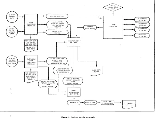
Figure

1 is a

graphical

representation

of the

methodology

used

to

produce

the

ancillary activity

models. In the _upper left cor-ner is the &dquo;Data

Processing Program&dquo;

which used both

patient

data and

ancillary

activity

data as

input.

A number of

inpatient

data items used

by

other _programs were

generated:

(1) All arrival rates and distributions needed to define and build the ASCSS models

(2) The

inpatient

portion

of the

ancillary

activity

measures

matrix

(3) The

patient

flow matrix used in the

production

of a run

reflecting

the _way the

hospital operated

in 1976.

The lower left-hand corner of

Figure

1 shows the _program that

processed

the _outpatient

ancillary

activity

data. It too was a

multipurpose

program and

produced:

(1) The

outpatient portion

of the

ancillary

activity

measures

matrix

(2) Hard copy

figures

detailing

the numbers of

outpatients

par-ticipating

in the

ancillary

activities under

study

(3) A MICRO formatted data set of

outpatient ancillary

activ-ity

to be used

eventually

in the

production

of

graphs.

The ASCSS

(upper

right-hand

corner of

Figure

1) functioned

in the

following

manner: For each scenario of

patient

flow

under

study,

a _separate model was constructed. Each model

was simulated as many times as _necessary until the simulation statistics reflected the desired

hospital

setting.

A

computation

program

(upper

middle of

Figure

1) was run

using

a different

patient

flow matrix each time to be

integrated

with the

inpatient

ancillary

activities measures matrix to

pro-duce MICRO formatted data sets with hard copy

statistics.’

Aggregation

of

graph

data resulted from the use of the MICRO

formatted data sets in

conjunction

with the MICRO

Informa-tion

Management

System.

From _{this program and the}

format-ted

data,

approximately

400 different sets of data were

pro-duced. Further

manipulation

was necessary before the

SOPH:GRAF and the SCH3:COMPOSE canned programs were

used to

produce

the 67

graphs

and

composite

graphs

of the

study.

RESULTS

AND

CONCLUSIONS

(1 )

Day

Of

Stay

Graphical

Summaries. For each of the 19

an-cillary

departments

of

interest,

graphical

summaries were

produced

that

displayed

the effect of

day

_{of stay} on

an-cillary

load.

Figure

2 is an

example

of the

inpatient

pro-cedure load on the

Biochemistry Laboratory

as a function

[image:4.606.47.550.58.442.2] [image:4.606.46.292.537.693.2]

Figure 1. _Activity simulation model.

a

relatively higher

load the first few

days

of _stay. Other

laboratories such as

Physical

Therapy (Figure

3) exhibited

a

procedure

load that was

higher

as the

day

of _stay

in-creased. Of the 19 laboratories of

interest,

14 exhibited

Figure 2. _{Average daily ancillary} load for Biochemistry Laboratory.

higher

loads the first few

days

of

stay (Table

1). This

obser-vation is somewhat

misleading,

as discussed

later,

because

the

impact

of

higher

loads was found to be

considerably

dampened by

the

&dquo;steady

state&dquo; loads that had to be met

every

day.

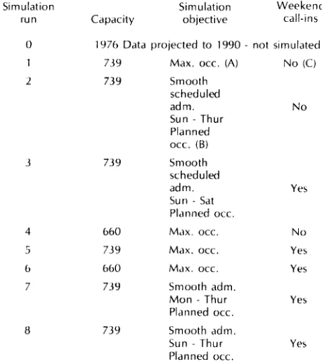
(2) The Effect Of

Varying Inpatient

Patient Flows. Table 2 de-fines the

experimental

scenarios for the simulation runs.

The

analysis

was

complicated by

the use of two bed

ca-pacities.

At this

point

in the

planning

_process, the number of beds that the

hospital

administration had decided to build

was 739. The minimum number needed to care for the

pre-dicted

patient

demand under _{maximum average occupancy}

considerations was determined to be 660. The

higher

number (739) gave much more

flexibility regarding

when

scheduled elective

patients

could be

admitted,

whereas the

lower number (660) gave no

flexibility

_except whether or

not _{urgent elective}

patients

were to be admitted on the

weekends.

Thus,

all except runs 4 and 6 used the 739 bed

capacity.

The &dquo;Smooth Scheduled Admissions&dquo; was an at-tempt to smooth the workload ori the

ancillary

services.

It was chosen as an

approach

because so _many of the

an-cillary departments

(14 of 19) had

higher procedure

loads

[image:5.606.54.302.51.236.2]

Figure 3. _{Average daily} ancillary load for Physical Therapy.

Table 1. A list of the laboratories _{having higher procedure} loads the first few

days of stay.

Approximate ratio of first or

second

day procedure

rate to

--

the average of the

following

18

a simulation but as the 1976 admission data transformed (LOS, admissions rate) to the 1990

planning

_year, so that

the

hospital

administration could compare any new

admis-sions

policies

with those

they

were

using

in 1976.

The weekend call-ins factor was included to show the ef-fect of the presence or absence of _urgent elective

admis-sions on weekends because some third _{party reimbursers}

were not

paying

for _urgent elective

patients

admitted on

weekends.

(3) The

Graphical

Output.

The

major

output

of the effort was a series of three

graphs

for each of the

ancillary

depart-ments : average

inpatient

procedure

load,

the _average

out-patient procedure load,

and the combined _average

pro-cedure load.

Examples

of these

graphs

are

presented

using

the

Biochemistry

Laboratory

as an

example

(Figures

4, 5,

and 6). In these

figures

the average number of

procedures

is

plotted

for each

day

of week for each of the simulation

runs. The numbers

superimposed

on the

graphs

are the

simulation run numbers of Table 2. For the

inpatient

and total

loads,

a relative scale is

presented along

the

right

side

with 100

being

the lowest

point,

so that one can _get an

idea of the relative

change

in load from

day

to

day,

which

is

presumed

to be related to staff size.

The

following

items _represent our conclusions

concerning

the

total

ancillary

loads:

A. The _{variation in average} load

by day

of week was different

for each of the

ancillary departments. Thus,

no

single

in-patient

admission

policy

would

provide

a stable workload

for all 19

departments.

B.

Outpatient

loads tended to mask and dominate variation in load due to

inpatient policies. Thus, outpatient

clinic

scheduling

was a critical _aspect of the

stability

for

ancillary

demands.

C. Maximum

occupancies

at the

planned

capacities

(739

beds)

gave much

higher

loads (runs 1 and 5) than loads

imposed

by projected

occupancies. Thus,

if 739 beds were to be

built,

ancillary

capacities

should be based on maximum

occupancy conditions not

planned

_occupancy conditions.

D. The differences in

inpatient

admissions

policies

were

primarily

reflected in total loads on

Saturday

and

Sunday

when

outpatient

demand was the lowest.

Table 2. A scenario _{of the inpatient simulation} runs.

Note: (A) Max. occ. is where

hospital

beds would be used to

maximum extent

subject

to scheduled admission cancellations and no beds for _emergency

con-stramts. This _gives an _upper bound to the use of

ancillary

tacilities.

(B) Planned occ. is the

planned

_occupancy for 1990.

(C) Weekend call-ins &dquo;no&dquo; is where urgent electives

[image:5.606.322.551.359.618.2]

[image:6.605.43.289.47.392.2]

Figure 4. Average number of inpatient procedures versus _day of the week for _{Biochemistry Laboratory} (for the simulation runs of Table 2).

E. The

generally higher

activity

of the

outpatient

departments

on

Monday

and

Tuesday

versus

Wednesday, Thursday

and

Friday

was

generally

reflected in the total load curves.

Thus,

if at all

possible,

outpatient activity

needed to be reduced

on

Monday

and

Tuesday

and increased on

Wednesday,

Thursday,

and

Friday

to smooth the total load.

F.

Preventing

weekend _urgent elective call-ins on

Friday

and

Saturday

decreased

ancillary

loads on

Friday

and

Saturday,

but

substantially

raised them on

Sunday,

so that _{in many}

ancillary departments, Sunday

had the

highest

load of _any

day

of the week.

G. Most of the

ancillary departments

are labor intensive so

that the number of

procedures

are

probably linearly

related to the staff

size,

both on an absolute and a relative basis.

Thus,

staffing

on a

daily

basis could be determined

using

the data of this

methodology

plus

the labor hours per

pro-cedure data for any

given ancillary

department.

Using

the

following

data as an

example

of

staffing

for the

Biochemistry

Laboratory:

(i) Let the load

predicted by

simulation run #8 be the

planned

load and the load

predicted by

run #5 be the

maximum load

(ii) Assume an _{average time per}

procedure

of 5.0 minutes

(iii)

Assume a 450.0 minute

working day.

Table 3

gives

the

required

staffs

by

day

of the week. Please note the

high staffing required

on

Saturday

and

Sunday

and

the differences between

planned

and maximum average

loads.

(4)

Outputs

versus Present Practice. A _{cursory examination of}

the

staffing

patterns

indicated

by

run 0

(1976

policies)

and the actual staff used in the

hospital

revealed a

tendency

to

substantially

understaff on weekends and to overstaff

on

Fridays.

These

practices

probably:

~

Substantially

raised the

ancillary

loads on

Monday

and

Tuesday,

which in many cases were

already relatively

high

due to

outpatient

policies.

if this demand is to be

met with full-time

staff,

overstaffing

toward the end of the week will occur if the units are

correctly

staffed

dur-ing

the first _part of the week.

~

Substantially

_{increased LOS due to the}

delay

_of

servic-ing

of _requests for service on the weekends.

~ _Caused

physicians

to minimize treatment on weekends

because of the poor

ancillary

response.

(5) Predictions of Weekend

Staffing

By Department.

Examina-tion

of Table

4,

which _compares

Monday

to

Friday

loads

versus

Saturday

and

Sunday

loads,

reveals that the [image:6.605.308.548.326.693.2]

staff-ing

on the weekend is

surprisingly high.

This result is due

Figure 5. Projected average number of procedures caused _{by outpatient}

[image:7.603.55.307.50.400.2]

Figure 6. Total average number of procedures (inpatient plus outpatient) for

Biochemistry Laboratory.

Table 3. Predicted _{average daily} staff at _planned and _{maximum average} load for the _{Biochemistry Laboratory.}

to the

&dquo;Steady

State Load&dquo; of many of the

ancillary

services

after the first few

days

of

stay

and to the

assumption

that

was made that the number of

procedures

for a

patient

was

due to _{the type of}

patient

and the

day

_{of stay,} not to the

day

of the week. This

assumption

was

justified

on the basis

that there was _great interest in

reducing

the LOS of

patients

and that one of the _ways to do this was to

provide

the same intensive service on weekends as

during

the week. If

staff-ing

is related

linearly

to

load,

then the

percent

figures

give

an indication of the

Saturday

and

Sunday

staff. The

follow-ing

is observed:

.

Saturday

_to

Sunday

_{staff varied between}

ancillary

depart-ments, but in all cases needed to be

higher

than

anticipated.

Table 4. A companson of the Saturday and Sunday average ancillary load with the Monday through Fnday load using simulation run #8 (from Table 2).

. _{Overall average is 80%} on

Sunday

and 74% on

Satur-day indicating

the weekend staffs needed to be

roughly

three-fourths of the staff

during

the week. This is

substan-tially

different than the

present

staffing

of the

hospital.

REFERENCES

1 DOWLING, W.

"Converting Demand Forecast into Facility Requirements." Cost Control in

Hospitals, Section 11.3. Health Administration Press, Ann Arbor, Michigan

(1976) 70-89.

2 DUMAS, B M. and STAPLETON, C. J.

"Hospital Bed _{Planning Via Computer} Simulation." Simulation in Health Care

Delivery Systems. The _Proceedings of the Conference on Simulation in Health

Care Delivery Systems, Simulation Councils, Inc., La Jolla, California (1983),

13-20.

3 GRIFFITH, J. R.; HANCOCK, W. M.; and MUNSON, F. C.

"Admission scheduling and control systems," Cost Control in _Hospitals, Sec-tion III.2. Health Administration Press, Ann Arbor, Michigan (1976), 150-185. 4 HANCOCK, W. M.; JOHNSON, C.; MAGERLEIN, D.; MARTIN, J.; and

WALTER, P.

Replacement Bed Size for University Hospital : Determination and Final Results. _Report No. 78-1. Management Information Systems Group of the

Department of Hospital Administration, The University of Michigan, Ann

Ar-bor _(May 1978).

5 HANCOCK, W. M. and WALTER, P. F.

The _{"ASCS" Inpatien}t Admission _Scheduling and Control _System. AUPHA Press,

Ann Arbor, Michigan (1983). 6 HANCOCK, W. M. and WALTER, P. F.

University Ancillary Services Project. Report 80-1, Management Information

Systems Group of the Department of Hospital Administration, University of Michigan (January 1980).

7 KAHN, M. A.; RUMELHART, D. _L., and BRONSON, B. L.

Micro Information _{Management System} Reference Manual. Institute of Labor

and Industrial Relations, The _{University of Michigan,} Ann Arbor, Michigan

(October 1977).

8 ROBINSON, G. H.; WING, P.; and DAVIS, L. E.

"Computer Simulation of Hospital Patient Scheduling Systems." Health

[image:7.603.319.549.69.311.2]