R E V I E W
Open Access
Lebesgue functions and Lebesgue
constants in polynomial interpolation
Bayram Ali Ibrahimoglu
**Correspondence:
bibrahim@yildiz.edu.tr Department of Mathematical Engineering, Yıldız Technical University, Davutpasa Campus, Istanbul, 34210, Turkey
Abstract
The Lebesgue constant is a valuable numerical instrument for linear interpolation because it provides a measure of how close the interpolant of a function is to the best polynomial approximant of the function. Moreover, if the interpolant is computed by using the Lagrange basis, then the Lebesgue constant also expresses the
conditioning of the interpolation problem. In addition, many publications have been devoted to the search for optimal interpolation points in the sense that these points lead to a minimal Lebesgue constant for the interpolation problems on the interval [–1, 1].
In Section 1 we introduce the univariate polynomial interpolation problem, for which we give two useful error formulas. The conditioning of polynomial interpolation is discussed in Section 2. A review of some results for the Lebesgue constants and the behavior of the Lebesgue functions in view of the optimal interpolation points is given in Section 3.
Keywords: polynomial interpolation; Lebesgue function; Lebesgue constant
1 Introduction Forn∈N, let
X={xj:j= , , . . . ,n} ()
be a set ofn+ distinct interpolation points (or nodes) on the real interval [–, ] such that
–≤x<x<· · ·<xn≤. ()
Let the functionf belong toC([–, ]). When approximatingf by an element from a finite-dimensionalVn=span{φ, . . . ,φn}withφi∈C([–, ]) for ≤i≤n, we know that there exists at least one elementp∗n∈Vnthat is closest tof. When using the · ∞norm, this element is the unique closest one if theφ, . . . ,φnare a Chebyshev system. Since the computation of this element is more complicated than that of the interpolant
n
i=
αiφi(xj) =f(xj), j= , . . . ,n, –≤xj≤,
there is an interest in interpolation pointsxjthat make the interpolation error
f(x) –
n
i= αiφi(x)
∞=xmax∈[–,]
f(x) –
n
i= αiφi(x)
as small as possible. In other words, there is an interest in using interpolating polynomials that are near-best approximants.
Whenφi(x) =xiandf is sufficiently differentiable, then for the interpolant
pn(x) = n
i= αixi
satisfyingpn(xj) =f(xj), ≤j≤n, the errorf–pn∞is bounded by [], pp.-
f–pn∞≤ max x∈[–,]
|f(n+)(x)| (n+ )!
max x∈[–,]
n
j=
|x–xj|. ()
In this study, we call this inequality the first error formula. It is well known that(x– x)· · ·(x–xn)∞is minimal on [–, ] if thexjare the zeroes of the (n+ )th-degree
Cheby-shev polynomialTn+(x) =cos((n+ )arccosx).
The operator that associates withf its interpolantpnis linear and given by
Pn[x, . . . ,xn] :C
[–, ] →Vn:f(x)→pn(x) = n
i=
f(xi)i(x), ()
where the basic Lagrange polynomials
i(x) = n
j=,i=j x–xj xi–xj
()
satisfyi(xj) =δij. So another bound for the interpolation error is given by
f–pn∞≤ +Pn f–p∗n∞, Pn=xmax∈[–,]
n
i=
i(x),
wherePn:=Pn[x, . . . ,xn] is the linear operator defined by (), andp∗nis the best uniform polynomial approximation tof.
2 Lebesgue function and constant
2.1 Definition and properties
Recall from () that
pn(x) = n
i=
f(xi)i(x),
For a fixednand givenx, . . . ,xn, the Lebesgue function is defined by
Ln(x) :=Ln(x, . . . ,xn;x) = n
i=
i(x),
and the Lebesgue constant is defined by
n:=n(x, . . . ,xn) = max –≤x≤
n
i=
i(x).
It is clear that bothLn(x) andndepend on the location of the interpolation pointsxj(and also on the degreen) but not on the function valuesf(xi). Note that the operator norm of Pndefined by () is equal to the∞-norm of its Lebesgue function:
Pn∞=n= max –≤x≤Ln(x).
Here and in the following, with the setXdefined by (), we sometimes writeLn(X;x) := Ln(x, . . . ,xn;x) andn(X) :=n(x, . . . ,xn) to simplify the notation.
The following present some basic properties of Lebesgue functions for Lagrange inter-polation (see,e.g., [, ]):
(a) For any setX, withn≥,Ln(X;x) is a piecewise polynomial satisfyingLn(X;x)≥ with equality only at the interpolation pointsxj,j= , . . . ,n.
(b) On each subinterval (xj–,xj) for ≤j≤n,Ln(X;x) has precisely one local maximum, which is denoted byλj(X). If the endpoints – and + are not interpolation points, that is, – <xandxn< , then there are two other subintervals and, thus, two other local maxima that are at –, and +. We denote the latter two local maxima byλ(X) andλn+(X).
(c) The greatest and the smallest local maxima ofLn(X;x) are denoted correspondingly byMn(X) andmn(X); we denote byδn(X) the maximum deviation among the local max-imaδn(X) =Mn(X) –mn(X). We also denote the position of the Lebesgue constant (by taking one of the greatest local maxima) byx∗(X) for the set of interpolation pointsX.
(d) The equalityLn(X;x) =Ln(X; –x),x∈[–, ], holds if and only ifxn–j= –xj,j= , . . . ,n. (e) The Lebesgue constant is invariant under the linear transformationtj=axjˆ +bˆ,j= , . . . ,n(aˆ= ). Interpolation sets that include the endpoints of the interval as interpolation points are called canonical interpolation sets. LetXˆ denote a canonical interpolation set. In particular, we may construct a setXˆ obtained fromXby mapping [x,xn] onto [–, ] by the unique linear transformationti=axiˆ +bˆ,i= , . . . ,n, whereaˆandbˆare determined by – =axˆ +bˆand =axnˆ +bˆ. Here the setXˆ is also called the canonicalization of the setX. We can see that the Lebesgue constant forXˆ is [, ], pp.-
n(t, . . . ,tn) = max
x≤x≤xnLn(x, . . . ,xn;x)≤
max
–≤x≤Ln(x, . . . ,xn;x). We use these properties in the sequel.
2.2 Importance of Lebesgue constants
One motivation for investigating the Lebesgue constant is that another upper bound for the interpolation error is given by
wherep∗nis the best polynomial approximation tof on [–, ], and thereforenquantifies how much larger the interpolation errorf –pn∞ is compared to the smallest possible
errorf –p∗n∞ in the worst case. In this study, we call this inequality the Lebesgue
in-equality or the second error formula.
It is easy to show how to obtain this inequality. From the uniqueness of the interpolat-ing polynomial we havepn(x) =ni=f(xi)i(x) andp∗n(x) =
n
i=p∗n(xi)i(x). By subtracting pn(x) fromp∗n(x) we get
p∗n(x) –pn(x)=
n
i=
p∗n(xi)i(x) – n
i=
f(xi)i(x)
=
n
i=
p∗n(xi) –f(xi) i(x)
≤
n
i=
i(x)max i=,...,n
p∗n(xi) –f(xi).
From this it follows that (due toLn(x) = n
i=|i(x)|) p∗n–pn∞≤nf–p∗n∞.
Finally, we have
f–pn∞=f–p∗n+p∗n–pn∞
≤f –p∗n∞+p∗n–pn∞
≤f –p∗n∞+nf–p∗n∞
= ( +n)f –p∗n∞.
As a simple consequence of this inequality, it is obvious thatpn→f as the factornf – p∗n∞→. Namely, the Lebesgue inequality indicates that for the interpolation of a fixed functionf on [–, ], convergence can be expected only iff is smooth enough such that
f–p∗n∞decreases, asn→ ∞, faster thannincreases.
Another motivation for investigating the Lebesgue constant is that the Lebesgue con-stant also expresses the conditioning of the polynomial interpolation problem in the La-grange basis. Letpn˜ (x) denote the polynomial interpolant of degreenfor the perturbed functionf˜in the same interpolation points:
˜
pn(x) = n
i=
˜
f(xi)i(x).
Sincepn∞≥maxi=,...,n|f(xi)|, we have
pn–pn˜ ∞
pn∞
≤maxx∈[–,]
n
i=|f(xi) –f˜(xi)||i(x)| maxi=,...,n|f(xi)|
≤n(x, . . . ,xn)
maxi=,...,n|f(xi) –f˜(xi)| maxi=,...,n|f(xi)|
This indicates that if we are able to choose interpolation points such thatnis small, then we can find the Lagrange interpolant that is less sensitive to errors in the function values. For this reason, numerical interpolation in floating-point arithmetic will generally be useless, even for smooth functionsf, whenever the Lebesgue constantnis larger than the inverse of the machine precision, which is typically about .
3 Some specific sets of interpolation points
This section gives a summary of some results for particular sets of interpolation points for which the behavior of the Lebesgue function has been well investigated.
3.1 Equidistant nodes
There are many studies on the behavior of the Lebesgue function corresponding to the set of equidistant points although this set is a bad choice for polynomial interpolation owing to the Runge phenomenon.
For the set of equidistant points
E=
xj= – + j
n,j= , , . . . ,n
, ()
the Lebesgue constantn(E) grows exponentially with the asymptotic estimate [, ]
n(E)
n+
en(logn+γ), n→ ∞, ()
where
γ = lim n→∞
n
i= i –logn
= . . . .
is Euler’s constant (or the Euler-Mascheroni constant). Also, an asymptotic expansion that improves () (with unknown explicit general formula for the series coefficients) is found in [].
Forn(E), the upper and lower bounds n–
n <n(E) < n+
n , n≥, ()
have been suggested []. In [], an upper bound is given for the smallest local maxima mn(E):
mn(E) <
π
log(n+ ) +log +γ . ()
Figure 1 Graphs ofL5(E;x) (left),L5(T;x) (center),L5(ˆT;x) (right).
Figure 2 6 Chebyshev ( ) and extended Chebyshev ( ) nodes.
subinterval (or due to symmetry in the last subinterval). Numerical observation shows that the location of the Lebesgue constant occurs near the midpoint of the last (or first) subinterval, that is,x∗(E)≈(n– )/nfor the interval [–, ].
From the Lebesgue inequality () we know that equidistant points with this very fast growth of the Lebesgue constant give very poor approximations asnincreases. Indeed, numerical experiments show that for degreen≥, the Lebesgue constantn(E) reaches the inverse of the machine precision.
3.2 Chebyshev nodes of the first kind
The literature describes numerous investigations for the behavior of the Lebesgue function corresponding to the set of Chebyshev nodes. They are a very good choice of points for polynomial interpolation, and as it was indicated in Section , they give the smallest upper bound for the interpolation error of polynomial interpolation. As illustrated in Figure , they are obtained by projecting equally spaced points on a semicircle down to the unit interval [–, ]; see the explicit formula ().
The set of Chebyshev points
T=
xj= –cos
π
(j+ )
(n+ )
,j= , , . . . ,n
()
is distributed more densely toward the endpoints of the interval [–, ], as illustrated in Figure forn= .
The Lebesgue constantn(T) for polynomial interpolation grows logarithmically with the asymptotic expression []
n(T) =
π
log(n+ ) +γ +log
π
+αn, <αn<
π
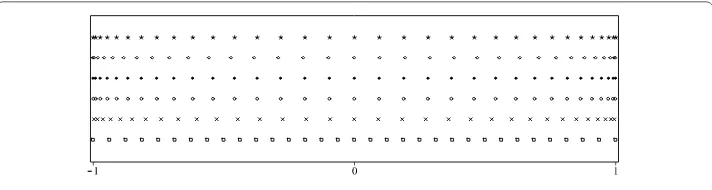
Figure 3 Graphs of sets of 33 nodes; (∗)˘T, ()¯U, (•)ˆT, (◦)T, (×)U, ()Efrom top to bottom.
from which the upper and lower bounds
πlog(n+ ) + . . . . <n(T) <
πlog(n+ ) + . . . . , n≥ ()
can be deduced.
Forn(T), an asymptotic series expansion, which is valid for all finiten, is given by [–]
n(T) =
π
log(n+ ) +γ +log
π
+
∞
v=
Av
(n+ )v, n≥,
where the coefficientsAvhave alternating signs and can be calculated as
Av= (–)v–
π
– –v
(π)v (v– )!ζ(v) ⎛ ⎝ +
∞
j=v+ ζ(j) ()j–
j– v–
⎞ ⎠,
where
ζ(s) =
∞
k= ks
is the Riemann zeta function.
Using the little-onotation defined byε(n) =o(e(n)) whenε(n)/e(n)→,n→ ∞, Brut-man showed [] that
mn(T) =n
(T) +o(), n≥, from which the lower bound
πlog(n+ ) +
π
log
π+γ
....
<mn(T)
is obtained. Later, this bound was improved [] as follows:
π
log(n+ ) +log
π +γ
+ π
(n+ ) –
π
A comparison of () and () shows that the deviation between any two local maxima of the Lebesgue functionLn(T;x) does not exceed .. This result was improved in [] to
δn(T) =Mn(T) –mn(T)≤
πlog = ..
As Figure (center) suggests, the local maxima ofLn(T;x) are decreasing strictly from the outside toward the midpoint of the interval [–, ], which was proven in []. The figure also shows that the location of the Lebesgue constant occurs at±, that is,x∗(T) =± [, ].
We know from the first error formula () that the Chebyshev points are a good choice for polynomial interpolation. Now, this slow growth of the Lebesgue constant confirms that they are also a good choice for the second error formula (), which becomes
f–pn∞≤
πlog(n+ ) +
f–p∗n∞
for the Chebyshev nodes. For example, forn= , the interpolation error based on the Chebyshev points is
f–pn∞≤.× f–p∗n∞,
that is, even in the worst case, the interpolation errorf –pn∞is only . times larger than the smallest possible error. For comparison, if we choose equidistant points for the same degree, then the upper bound for the interpolation error is
f–pn∞≤.× f –p∗n∞.
3.3 Extended Chebyshev nodes
The extended Chebyshev nodesTˆ are defined by
ˆ
T=
xj= –cos
π
(j+ )
(n+ )
cos
π
(n+ )
,j= , , . . . ,n
,
where the division by cos(π/(n+ )) guarantees thatx= – andxn= , and the setTˆ is obtained from the set T by the linear transformation that maps [x,xn] onto [–, ]. Therefore, the setTˆ is the canonicalization of the Chebyshev setT(see Figures and ). From the monotonicity result for the local maxima ofLn(T;x) and property (e) given in Section . [, ],
max x<x<xn
Ln(x, . . . ,xn;x)≤ max
–≤x≤Ln(x, . . . ,xn;x),
Lebesgue constant for the extended Chebyshev nodes is given by []
n(Tˆ) =
π
log(n+ ) +γ +log
π
–
π +βn,
<βn<
.
log((n+ )/),n≥. ()
Hence, we can derive the upper and lower bounds
πlog(n+ ) + . . . . <n(Tˆ) <
πlog(n+ ) + . . . . , n≥.
Also, an asymptotic expansion ofβn(with unknown explicit general formula for the series coefficients, in contrast to the Chebysev nodes) can be found in [].
As for the maximum deviationMn(Tˆ) –mn(Tˆ) of the extended Chebyshev nodes, the following estimate is given []:
δn(Tˆ) =Mn(Tˆ) –mn(Tˆ)≤., n≥.
From () together with () it follows that this maximum deviation converges to
lim
n→∞δn(Tˆ) = . . . . .
3.4 Chebyshev extrema
The Chebyshev extremaU¯ are the zeros of the polynomial ( –x)T
n(x) and are given in explicit form as
¯
U=
xj= –cos
jπ
n
,j= , , . . . ,n
.
The Lebesgue constantn(U¯) for polynomial interpolation is [, ]
n(U¯) = ⎧ ⎨ ⎩
n–(T), nodd,
n–(T) –αn, <αn<n,neven.
It is shown in [] that the smallest local maximamn(U¯) are bounded (in contrast to the case of the Chebyshev nodesT) by
mn(U¯) < . . . . .
Thus, as in the case of the setE,n(U¯) andmn(U¯) are of different orders of magnitude, and the maximum deviation of the local maximaδn(U¯) tends to infinity logarithmically.
As was proven in [], the local maxima ofLn(U¯;x) increase strictly monotonically from the outside toward the midpoint of the interval [–, ]. This behavior suggests that the Lebesgue functionLn(U¯;x) achieves its maximum value on the subinterval (xn/,x(n+)/) (or its mirror) for even degrees and on the subinterval (x(n–)/,x(n+)/) for odd degrees.
3.5 Chebyshev nodes of the second kind
The Chebyshev nodes of the second kindUare the zeros of the (n+ )th-degree Chebyshev polynomial of the second kind
Un+(x) =
sin((n+ )arccos(x)) sin(arccos(x)) and are given in closed form by
U=
xj= –cos
(j+ )π
n+
,j= , , . . . ,n
.
For the Lebesgue constant, it is known thatn(U) =O(n) [], pp.-. In [], an exact expression forn(U) is given by
n(U) =n+ ,
and a lower bound formn(U) is given by
πlog(n+ ) + . . . . <mn(U).
Thus, as in the cases of the setsE andU¯,n(U) andmn(U) are of different orders of magnitude. In this case, the maximum deviation of the local maximaδn(U) has a linear growth.
Note that these interpolation points can be obtained from the zeros of the polynomial ( –x)T
n+(x) by deleting the zeros±. Thus, it follows that the Lebesgue constants are sensitive to the deletion of the endpoints.
3.6 Fekete nodes
Since the basic Lagrange polynomialsi(x) can be expressed with the quotient of two Van-dermonde determinants, namely
i(x) =|
V(x, . . . ,xi–,x,xi+, . . . ,xn)|
|V(x, . . . ,xn)|
, V(x, . . . ,xi, . . . ,xn) =
⎛ ⎜ ⎜ ⎜ ⎜ ⎜ ⎜ ⎜ ⎜ ⎝
x . . . xn ..
. ... xi . . . xn
i ..
. ... xn . . . xnn
⎞ ⎟ ⎟ ⎟ ⎟ ⎟ ⎟ ⎟ ⎟ ⎠ ,
we can expect that the interpolation points maximizing the Vandermonde determinant
|V(x, . . . ,xn)|yield a small Lebesgue constant. This node set is given by
–x dQn dx (x) =
For the Lebesgue constantn(F), we havei(x)∞≤ for ≤i≤n, and thus the
cor-responding Lebesgue constant is bounded by (at most) the dimension of the interpolation space:
n(F) = max –≤x≤
n
i=
i(x)≤n+ .
Moreover [], the Fekete points minimizemax–≤x≤
n
i=(i(x)), and for these points, max–≤x≤ni=(i(x))= . From this, by applying the Cauchy-Schwartz inequality,
n(F)≤
√
n+ .
This upper bound, however, is very pessimistic. In [], an improved upper bound for
n(F) is given by
n(F)≤clog(n+ )
with undetermined positive constantc. In addition [], based on numerical experiments, the estimate
n(F)≤
πlog(n+ ) + .
was conjectured. Accordingly, this confirms the conjecture in [] that
n(Tˆ) <n(F) <n(T), n≥.
3.7 Optimal nodes
The set of interpolation points is said to be optimal if it minimizes the Lebesgue constant. We denote the set of optimal nodes byX∗(or the Lebesgue-optimal point set in [–, ]):
n
X∗ =min X n(X).
Owing to the second error formula () and also formula () (for sensitivity to perturbations in the function values), it is desirable to minimize the Lebesgue constant. However, the set of optimal nodes on the interval [–, ] is known explicitly only for degrees less than four [, ], although their characterization is known from the Bernstein-Erdös conjectures. In , Bernstein [] conjectured that the greatest local maximum of the Lebesgue function is minimal whenLn(x) equioscillates, that is,
λ
X∗ =λ
X∗ =· · ·=λn
X∗ .
Later, Erdös [, ] added to this conjecture that there is a unique canonical setXˆ∗for which the smallest local maximum achieves its maximum. This is the case where the local maximum values are equal or, in other words,
mn(X)≤mnX∗ =n
X∗ =Mn
These conjectures were proven by Kilgore [, ] and by de Boor and Pinkus []. They showed that for degreen, the optimal canonical interpolation set is unique, symmetric, and that its Lebesgue function must necessarily equioscillate. By using these basic prop-erties of the optimal nodes a numerical procedure based on a nonlinear Remez search and exchange algorithm is given to compute the optimal nodes for polynomial interpolation on [–, ] []. Moreover, many authors (see,e.g., [, ]) have investigated (near) optimal point sets (in different norms) defined by the solutions of certain optimization problems. The first sharp estimate for the optimal Lebesgue constant is given by Vértesi []. By constructing the following modification of the Chebyshev nodes asymptotically optimal upper and lower bounds are given [–], pp.-. Let us denote this set by
˘
T=
xj= – cos(
π
(j+) (n+)) cos( π
(n+)( + log(n+)))
,j= , . . . ,n– ,xn= –x=
.
The Lebesgue constantn(T˘) satisfies
c
log log(n+ ) log(n+ )
>n(T˘) –
π
log(n+ ) +γ+log
π
>
π
(n+) +O((n+) ), nodd, –π(n+)+O((n+ )), neven,
wherecis an undetermined positive constant.
An application of the Erdös inequality (), combined with the lower bound formn(T) () and the upper bound forn(T˘), gives
π
(n+ )+O
(n+ )
<n
X∗ –
π
log(n+ ) +γ +log
π
< c
log log(n+ ) log(n+ )
.
From this we can deduce that the precise growth formulas for n(X∗) andn(T˘) are, respectively,
n
X∗ =
π
log(n+ ) +γ +log
π
+o()
and
n(T˘) =
π
log(n+ ) +γ +log
π
+o().
Sincen(T˘) andn(X∗) have the same asymptotic growth, we can conclude that the set
˘
T has asymptotically minimal Lebesgue constants.
At this point, some remarks are useful. From () we can derive a precise growth formula forn(Tˆ):
n(Tˆ) =
Table 1 The values of the maximum deviations and Lebesgue constants for setsT˘,Tˆ, andX∗
n setT˘ setTˆ setX∗
δn(T)˘ n(T)˘ δn(T)ˆ n(T)ˆ n(X∗)
10 0.050 781 2.056 087 0.019 471 2.068 744 2.051 706
20 0.056 995 2.463 129 0.019 340 2.479 193 2.460 788
40 0.061 827 2.887 067 0.018 952 2.904 441 2.885 809
Figure 4 Graphs ofL10(ˆT;x),L10(˘T;x),L10(X∗;x) from left to right.
Comparingn(Tˆ) andn(T˘), we can see that the setT˘ is better than the setTˆ in min-imizing Lebesgue constant. Indeed, numerical results confirm this (see Table and also Figure ). The maximum deviation of the nodal setT˘ converges to (see [], ())
lim
n→∞δn(T˘) = . . . . .
Hence, we conclude that the nodal sets studied in this section can be ordered with re-spect to their maximum deviationδn(X) =Mn–mn(X) and their Lebesgue constantn(X) in the following way:
δn(E) >δn(U) >δn(U¯) >δn(T) >δn(T˘) >δn(Tˆ) >δn
X∗ =
and
n(E) >n(U) >n(T) >n(U¯) >n(F) >n(Tˆ) >n(T˘) >n
X∗ .
4 Concluding remarks
In this paper we work with the interval [–, ] although all results on polynomial interpo-lation may be applied to any finite interval by a linear change of variable.
In view of the optimal interpolation points for the univariate polynomial interpolation, to our knowledge, both setsT˘ andTˆ, with the position of the points given in explicit form, are the best nodal sets in the literature. Based on the Bernstein-Erdös conjecture, the nodal setTˆ is superior than the nodal setT˘ because of its smaller maximum deviation. When considering the optimality of a nodal set from its Lebesgue constant, the setT˘ is better.
proved in []. No configurations of interpolation points obeying this order of growth are known. On the simplex, the minimal order of growth is not even known.
Competing interests
The author declares that he has no competing interests.
Acknowledgements
The author expresses his sincere thanks to Professor Annie Cuyt for her kind suggestions. This work was partially supported by the Scientific and Technical Research Council of Turkey (TUBITAK) under Grant No. 2214/B.
Received: 7 July 2015 Accepted: 20 February 2016
References
1. Davis, PJ: Interpolation and Approximation. Blaisdell, New York (1963)
2. Luttmann, FW, Rivlin, TJ: Some numerical experiments in the theory of polynomial interpolation. IBM J. Res. Dev.9, 187-191 (1965)
3. Brutman, L: Lebesgue functions for polynomial interpolation - a survey. Ann. Numer. Math.4(1-4), 111-127 (1997) 4. Phillips, GM: Interpolation and Approximation by Polynomials. CMS Books in Mathematics [Ouvrages de
Mathématiques de la SMC], vol. 14, p. xiv+312. Springer, New York (2003) 5. Schönhage, A: Fehlerfortpflanzung bei Interpolation. Numer. Math.3, 62-71 (1961)
6. Turetskii, H: The bounding of polynomials prescribed at equally distributed points. Proc. Pedag. Inst. Vitebsk3, 117-121 (1940) (in Russian)
7. Mills, TM, Smith, SJ: The Lebesgue constant for Lagrange interpolation on equidistant nodes. Numer. Math.61(1), 111-115 (1992)
8. Trefethen, LN, Weideman, JAC: Two results on polynomial interpolation in equally spaced points. J. Approx. Theory
65(3), 247-260 (1991)
9. Tietze, H: Eine Bemerkung zur Interpolation. Z. Angew. Math. Phys.64, 74-90 (1917) 10. Günttner, R: Evaluation of Lebesgue constants. SIAM J. Numer. Anal.17(4), 512-520 (1980)
11. Dzjadik, VK, Ivanov, VV: On asymptotics and estimates for the uniform norms of the Lagrange interpolation polynomials corresponding to the Chebyshev nodal points. Anal. Math.9(2), 85-97 (1983)
12. Shivakumar, PN, Wong, R: Asymptotic expansion of the Lebesgue constants associated with polynomial interpolation. Math. Comput.39(159), 195-200 (1982)
13. Brutman, L: On the Lebesgue function for polynomial interpolation. SIAM J. Numer. Anal.15(4), 694-704 (1978) 14. Günttner, R: Note on the lower estimate of optimal Lebesgue constants. Acta Math. Hung.65(4), 313-317 (1994) 15. Ehlich, H, Zeller, K: Auswertung der Normen von Interpolationsoperatoren. Math. Ann.164, 105-112 (1966) 16. Powell, MJD: On the maximum errors of polynomial approximations defined by interpolation and by least squares
criteria. Comput. J.9, 404-407 (1967)
17. Günttner, R: On asymptotics for the uniform norms of the Lagrange interpolation polynomials corresponding to extended Chebyshev nodes. SIAM J. Numer. Anal.25(2), 461-469 (1988)
18. McCabe, JH, Phillips, GM: On a certain class of Lebesgue constants. Nordisk. Tidskr. Informationsbehandling (BIT)13, 434-442 (1973)
19. Szeg ˝o, G: Orthogonal Polynomials, 3rd edn., p. xiii+423. Am. Math. Soc., Providence (1967)
20. Fejér, L: Bestimmung derjenigen Abszissen eines Intervalles, für welche die Quadratsumme der Grundfunktionen der Lagrangeschen Interpolation im Intervalle ein Möglichst kleines Maximum Besitzt. Ann. Sc. Norm. Super. Pisa, Cl. Sci.
1(3), 263-276 (1932)
21. Sündermann, B: Lebesgue constants in Lagrangian interpolation at the Fekete points. Mitt. Math. Ges. Hamb.11(2), 204-211 (1983)
22. Hesthaven, JS: From electrostatics to almost optimal nodal sets for polynomial interpolation in a simplex. SIAM J. Numer. Anal.35(2), 655-676 (1998)
23. Rack, HJ: An example of optimal nodes for interpolation. Int. J. Math. Educ. Sci. Technol.15(3), 355-357 (1984) 24. Rack, HJ: An example of optimal nodes for interpolation revisited. In: Advances in Applied Mathematics and
Approximation Theory. Springer Proc. Math. Stat., vol. 41, pp. 117-120. Springer, New York (2013)
25. Bernstein, S: Sur la limitation des valeurs d’un polynômePn(x) de degrénsur tout un segment par ses valeurs en (n+ 1) points du segment. Izv. Akad. Nauk SSSR7, 1025-1050 (1931)
26. Erdös, P: Problems and results on the theory of interpolation. I. Acta Math. Acad. Sci. Hung.9, 381-388 (1958) 27. Erdös, P: Some remarks on the theory of graphs. Bull. Am. Math. Soc.53, 292-294 (1947)
28. Kilgore, TA: Optimization of the norm of the Lagrange interpolation operator. Bull. Am. Math. Soc.83(5), 1069-1071 (1977)
29. Kilgore, TA: A characterization of the Lagrange interpolating projection with minimal Tchebycheff norm. J. Approx. Theory24(4), 273-288 (1978)
30. De Boor, C, Pinkus, A: Proof of the conjectures of Bernstein and Erdös concerning the optimal nodes for polynomial interpolation. J. Approx. Theory24(4), 289-303 (1978)
31. Angelos, JR, Kaufman, EH, Henry, MS, Lenker, TD: Optimal nodes for polynomial interpolation. In: Chui, CK, Schumaker, LL, Ward, JD (eds.) Approximation Theory. VI, pp. 17-20. Academic Press, New York (1989)
32. Chen, Q, Babuška, I: Approximate optimal points for polynomial interpolation of real functions in an interval and in a triangle. Comput. Methods Appl. Mech. Eng.128(3-4), 405-417 (1995)
36. Bos, L, De Marchi, S, Caliari, M, Vianello, M, Xu, Y: Bivariate Lagrange interpolation at the Padua points: the generating curve approach. J. Approx. Theory143(1), 15-25 (2006)
37. Bos, L, De Marchi, S, Vianello, M: On the Lebesgue constant for the Xu interpolation formula. J. Approx. Theory141(2), 134-141 (2006)