Several new inequalities for the minimum eigenvalue of M matrices

(1)

R E S E A R C H

Open Access

Several new inequalities for the minimum

eigenvalue of

M

-matrices

Jianxing Zhao

*

_{and Caili Sang}

*_{Correspondence:}

[email protected]

College of Science, Guizhou Minzu University, Guiyang, Guizhou 550025, P.R. China

Abstract

Several convergent sequences of the lower bounds for the minimum eigenvalue of M-matrices are given. It is proved that these sequences are monotone increasing and improve some existing results. Finally, numerical examples are given to show that these sequences are better than some known results and could reach the true value of the minimum eigenvalue in some cases.

MSC: 15A06; 15A15; 15A48

Keywords: M-matrix; nonnegative matrix; Hadamard product; spectral radius; minimum eigenvalue

1 Introduction

For a positive integern,Ndenotes the set{, , . . . ,n}, andRn×n₍_Cn×n_{) denotes the set of all}

n×nreal (complex) matrices throughout. ForA= [aij]∈Rn×n, we writeA≥ (A> ) if

allaij≥ (aij> ),i,j∈N. IfA≥ (A> ), we sayAis nonnegative (positive, respectively).

LetZndenote the class of alln×nreal matrices all of whose oﬀ-diagonal entries are

nonpositive. A matrixAis called a nonsingularM-matrix if A∈Zn and the inverse of

A, denoted byA–_{, is nonnegative. Denote by} _M

n the set of alln×nnonsingular

M-matrices (see []). IfAis a nonsingularM-matrix, then there exists a positive eigenvalue of Aequal toτ(A) =ρ(A–)–, whereρ(A–) is the Perron eigenvalue of the nonnegative ma-trixA–_{. It is easy to prove that}_τ_{(A) =}_min_{|_λ_|_:_λ_∈_σ_(A)_}_{, where}_σ_{(A) denotes the}

spec-trum ofA.τ(A) is called the minimum eigenvalue ofA(see []). The Perron-Frobenius theorem tells us thatτ(A) is an eigenvalue ofAcorresponding to a nonnegative eigenvec-torx= [x,x, . . . ,xn]T. If, in addition,Ais irreducible, thenτ(A) is simple andx>  (see

[]). IfGis the diagonal matrix of anM-matrixA, then the spectral radius of the Jacobi iterative matrixJA=G–(G–A) ofA, denoted byρ(JA), is less than  (see []).

A matrixAis called reducible if there exists a nonempty proper subsetI⊂Nsuch that aij= ,∀i∈I,∀j∈/I. IfAis not reducible, then we callAirreducible (see []).

For two real matricesA= [aij] andB= [bij] of the same size, the Hadamard product of

AandBis deﬁned as the matrixA◦B= [aijbij]. IfA∈MnandB≥, then it is clear that

B◦A–_≥_{ (see []).}

(2)

For convenience, we employ the following notations throughout. LetA= [aij]∈Mnwith

aii=  for alli∈N, andA–= [αij]. Fori,j,k∈N,j=i, denote

Ri(A) = n

j=

aij, M=max

i∈N n

j=

αij, M=min

i∈N n

j=

αij; σi=

j=i|aij|

|aii|

,

σ=max

i∈N σi, ϕi=

 aii–

k=i|aik|σk

; ri=max j=i

_|

aji|

|ajj|–

k=j,i|ajk|

,

mji=

|aji|+

k=j,i|ajk|ri

|ajj|

, hi=max j=i

_|

aji|

|ajj|mji–

k=j,i|ajk|mki

,

uji=

|aji|+

k=j,i|ajk|mkihi

|ajj|

, ui=max j=i {uij}.

Recall thatA= [aij]∈Cn×nis called row diagonally dominant ifσi≤ for alli∈N. If

σi< , we say thatAis strictly row diagonally dominant. It is well known that a strictly row

diagonally dominant matrix is nonsingular.Ais called weakly chained diagonally domi-nant ifσi≤,J(A) ={i∈N:σi< } =∅and for alli∈N/J(A), there exist indicesi,i, . . . ,ik

inNwithailil+= , ≤l≤k– , wherei=iandik∈J(A). Notice that a strictly diagonally dominant matrix is also weakly chained diagonally dominant (see []).

Estimating the bounds for the minimum eigenvalue ofM-matrices is an interesting sub-ject in matrix theory, it has important applications in many practical problems (see []), and various reﬁned bounds can be found in [–]. Hence, it is necessary to estimate the bounds forτ(A).

In [], Shivakumaret al.obtained the following bounds forτ(A): LetA= [aij]∈Rn×nbe

a weakly chained diagonally dominantM-matrix,A–_{= [}_α

ij]. Then

min

i∈N Ri(A)≤τ(A)≤maxi∈N Ri(A), τ(A)≤mini∈N aii and

 M

≤τ(A)≤  M

. ()

Subsequently, Tian and Huang [] provided a lower bound forτ(A) using the spectral radius of the Jacobi iterative matrixJAofA: LetA= [aij]∈MnandA–= [αij]. Then

τ(A)≥ 

[ + (n– )ρ(JA)]maxi∈Nαii

. ()

Furthermore, whenAis a strictly diagonally dominantM-matrix, they presented a lower bound forτ(A) which depends only on the entries ofA: IfA= [aij]∈Mnis strictly row

diagonally dominant, then

τ(A)≥ 

[ + (n– )σ]maxi∈Nϕi

. ()

In , Liet al.[] improved () and (), and they gave the following result: LetA= [aij]∈MnandA–= [αij]. Then

τ(A)≥ 

maxi=j{αii+αjj+ [(αii–αjj)+ (n– )αiiαjjρ(JA)]

 }

(3)

Furthermore, whenAis a strictly diagonally dominantM-matrix, they also presented a lower bound forτ(A) which depends only on the entries ofA: IfA= [aij]∈Mnis strictly

row diagonally dominant, then

τ(A)≥ 

max_i=j{ϕi+ϕj+ [ϕij+ (n– )ϕiϕjσ]

 }

, ()

whereϕij=max{ϕi,ϕj}–min{a–ii ,a–jj }.

In , Wang and Sun [] presented the following result: LetA= [aij]∈MnandA–=

[αij]. Then

τ(A)≥ 

maxi=j{αii+αjj+ [(αii–αjj)+ (n– )αiiαjjuiuj]

 }

. ()

And they gave examples to show that () is better than () and ().

In this paper, we continue to research the problems mentioned above and give some con-vergent sequences for the lower bounds of the minimum eigenvalue ofM-matrices which improve ()-(). Finally, numerical examples are given to verify the theoretical results.

2 Main results

In this section, we present our main results. First of all, we give some notations and lem-mas. LetB≥,D=diag(bii) andD=diag(dii), wheredii=  ifbii= ;dii=biiifbii= .

DenoteJB=D– (B–D), thenρ(JBT) =ρ(J_B) (see []).

LetA= [aij]∈Rn×n,aii= , i∈N. Fori,j,k∈N,j=i,t= , , . . . , denote

u()_ji =uji, p(jit)=

|aji|+

k=j,i|ajk|u(kit–)

|ajj|

, p(_it)=max j=i

p(_ijt),

h(_it)=max j=i

_|

aji|

|ajj|p(jit)–

k=j,i|ajk|p(_kit)

, u(_jit)=|aji|+

k=j,i|ajk|p(kit)h

(t)

i

|ajj|

.

Similar to the proof of Lemma , Lemma , and Lemma  in [], we can obtain the following lemma.

Lemma  If A= [aij]∈Mnis strictly row diagonally dominant,then A–= [αij]exists,and

for all i,j∈N,j=i,t= , , . . . ,

(a)  >ri≥mji≥uji=u()ji ≥p

()

ji ≥u

()

ji ≥p

()

ji ≥u

()

ji ≥ · · · ≥p

(t)

ji ≥u

(t)

ji ≥. . .≥; (b) ≥hi≥,≥h(it)≥;

(c) αji≤p(jit)αii; (d) 

aii ≤αii≤



aii–

j=i|aij|p(jit)

=φ_i(t).

Lemma  [] If A– _{is a doubly stochastic matrix,} _{then Ae} ₌_e, _AT_e ₌_e, _{where e}₌

[, , . . . , ]T_.

Lemma [] Let A,B∈Rn×n,and let X,Y∈Rn×nbe diagonal matrices.Then

(4)

Lemma [] Let A= [aij]∈Cn×nand x,x, . . . ,xnbe positive real numbers.Then all the

eigenvalues of A lie in the region

i,j∈N,i=j

z∈C:|z–aii||z–ajj| ≤ xi

k=i

 xk

|aki| xj

k=j

 xk

|akj|

.

Theorem  Let A= [aij]∈Mn,n≥,B= [bij]≥,and A–= [αij].Then,for t= , , . . . ,

ρB◦A–≤  maxi=j

biiαii+bjjαjj+

(biiαii–bjjαjj)+ p(it)p

(t)

j αiiαjjdiidjjρ(JB)

 

= t. ()

Proof SinceAis anM-matrix, there exists a positive diagonal matrixX, such thatX–AX is a strictly row diagonally dominantM-matrix (see []), and

ρB◦A–=ρX–B◦A–X=ρB◦X–AX–.

Hence, for convenience and without loss of generality, we assume thatAis a strictly diag-onally dominant matrix.

(a) First, we assume thatAandBare irreducible matrices. SinceBis nonnegative and irreducible, and so isJBT. Then there exists a positive vectorx= (x_i) such thatJ_BTx=

ρ(J_BT)x=ρ(J_B)x, thus, we obtain _k₌_ib_kix_k =ρ(J_B)d_iix_i and_k₌_jb_kjx_k =ρ(J_B)d_jjx_j,

i,j∈N. LetX=diag(x,x, . . . ,xn), then

B= [bˆij] =XBX–=

⎡ ⎢ ⎢ ⎢ ⎢ ⎣

b b_x_x · · · b_xn_nx

bx

x b · · ·

bnx

xn

..

. ... . .. ...

bnxn

x

bnxn

x · · · bnn ⎤ ⎥ ⎥ ⎥ ⎥ ⎦.

From Lemma , we haveB◦A–_{= (XBX}–₎_◦_A–₌_X(B_◦_A–_)X–_{. Thus,} _ρ₍_B_◦_A–_{) =}

ρ(B◦A–_{). Let}_λ₌_ρ₍_B_◦_A–_{), then}_λ_≥_b

iiαii,∀i∈N. By Lemma , there arei,j∈N,i=j

such that

|λ–biiαii||λ–bjjαjj| ≤ p(it)

k=i

 p(_kt)

ˆ

bkiαki p(jt)

k=j

 p(_kt)

ˆ

bkjαkj

.

Note that

p(_it)

k=i



p(_kt)

ˆ

bkiαki≤p(it)

k=i



p(_kt)

ˆ

bkip(kit)αii≤p(it)

k=i



p(_kt)

ˆ

bkip(kt)αii

=p(_it)αii

k=i

ˆ

bki=p(it)αii

k=i

bkixk

xi

=p(_it)αiidiiρ(JB).

Similarly, we havep(_jt)_k₌_j 

p(_kt)bˆkjαkj=p

(t)

j αjjdjjρ(JB). Hence, we obtain

(λ–biiαii)(λ–bjjαjj)≤p(it)p

(t)

(5)

From (), we have

λ≤  

(t)

 _,

that is,

ρB◦A–≤  

(t)

 

≤ 

maxi=j

(t)

 _.

(b) Now, assume that one ofAandBis reducible. It is well known that a matrix inZn

is a nonsingularM-matrix if and only if all its leading principal minors are positive (see condition (E) of Theorem .. of []). If we denote byC= [cij] then×npermutation

matrix withc=c=· · ·=cn–,n=cn= , the remainingcijzero, then bothA–εCand

B+εCare irreducible matrices for any chosen positive real numberε, suﬃciently small such that all the leading principal minors of bothA–εCandB+εCare positive. Now we substituteA–εCandB+εCforAandB, in the previous case, and then lettingε→, the

result follows by continuity.

Theorem  The sequence{ t},t= , , . . .obtained from Theoremis monotone

decreas-ing with a lower boundρ(B◦A–₎_and,_{consequently,}_{is convergent.}

Proof By Lemma , we have  >p(_jit)≥p_ji(t+)≥,j,i∈N,j=i,t= , , . . . . Then, by the deﬁnition ofp(_it), it is easy to see that the sequence{p(_it)}is monotone decreasing, and so is{ t}. Hence, the sequence{ t}is convergent.

Theorem  Let A= [aij]∈Mnand A–= [αij].Then,for t= , , . . . ,

τ(A)≥ 

maxi=j{αii+αjj+ [(αii–αjj)+ (n– )p(it)p

(t)

j αiiαjj]

 }

=ϒt. ()

Proof Let all entries ofBin () be . Thenbii= ,∀i∈N,ρ(JB) =n– . Therefore, by (),

we have

τ(A) =  ρ(A–₎≥



maxi=j{αii+αjj+ [(αii–αjj)+ (n– )p(it)p

(t)

j αiiαjj]

 }

.

The proof is completed.

Similar to the proof of Theorem , we can obtain the following theorem.

Theorem  The sequence{ϒt},t= , , . . .obtained from Theoremis monotone

increas-ing with an upper boundτ(A)and,consequently,is convergent.

Remark  We next give a simple comparison between () and (). According to Lemma , we know that for alli,j∈N,j=i,t= , , . . . ,  >uji≥p(jit)≥. Furthermore, by the

deﬁni-tions ofui,p(it), we have  >ui≥p(it)≥. Obviously, fort= , , . . . , the bounds in () are

(6)

Next, we give lower bounds forτ(A) which depend only on the entries ofAwhenAis a strictly diagonally dominantM-matrix.

Corollary  If A= [aij]∈Mnis strictly diagonally dominant,then for t= , , . . . ,

τ(A)≥ 

maxi=j{φi(t)+φ

(t)

j + [(φ

(t)

ij )+ (n– )p

(t)

i p

(t)

j φ

(t)

i φ

(t)

j ]

 }

=t, ()

whereφ_ij(t)=max{φ(_it),φ_j(t)}–min{a–_ii ,a–_jj }.

Proof LetA–= [αij]. SinceA∈Mnis strictly diagonally dominant, by Lemma , we have

a_ii–≤αii≤φi(t), i∈N, ()

from which we get

(αii–αjj)≤

maxφ(_it),φ_j(t)–mina–_ii,a–_jj =φ_ij(t). () From inequalities (), (), and (), the conclusion follows.

Corollary  The sequence{t},t= , , . . .obtained from Corollaryis monotone

increas-ing with an upper boundτ(A)and,consequently,is convergent.

Theorem  Let A= [aij]∈Mnwith a=a=· · ·=ann,and suppose A–= [αij]is doubly

stochastic.Then,for t= , , . . . ,

ϒt≥



maxi=j{αii+αjj+ [(αii–αjj)+ (n– )αiiαjjρ(JA)]

 }

≥ 

[ + (n– )ρ(JA)]maxi∈Nαii

()

and

t≥



maxi=j{ϕi+ϕj+ [ϕij+ (n– )ϕiϕjσ]

 }

. ()

Proof Since A– _{is doubly stochastic, by Lemma , we have} _|_a

ii| =

k=i|aik| +  =

k=i|aki|+ . Then for everyi∈N,ri=maxl=i{_|_a_ll_|_–|ali|

k=l,i|alk|}=maxl=i{

|ali|

+|ali|}=

maxl=i|ali|

+maxl=i|ali|.

Sincef(x) = _+x_xis an increasing function on (, +∝), we have

ri=

maxl=i|ali|

 +maxl=i|ali|

≤

k=i|aki|

 +_k₌_i|aki|

=

k=i|aki|

|aii|

=  – 

|aii|

, i∈N.

Furthermore, note that

JA=

⎡ ⎢ ⎢ ⎢ ⎢ ⎣

 –a

a · · · –

an

a –a

a  · · · –

an

a ..

. ... . .. ... –an

ann –

an

ann · · · 

(7)

is a nonnegative matrix and

k=i|aik|

|aii| =  –



|aii|, i∈N. Hence, by the Perron-Frobenius

theorem [], we haveρ(JA) =  –_|_a_ii_|,i∈N.

Combining with Lemma , we have, for alli,j∈N,j=i,t= , , . . . ,  >ρ(JA)≥ri≥uji≥

p(_jit)≥. By the deﬁnitions ofui,p(it), we have

 >ρ(JA)≥ri≥ui≥p(it)≥, i∈N.

Obviously, by inequalities (), (), and Theorem . of [], the inequality () holds. The

inequality () is proved similarly.

3 Numerical examples

In this section, several numerical examples are given to verify the theoretical results.

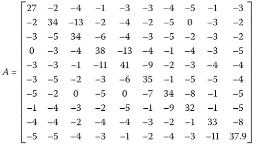
Example  Let

A= ⎡ ⎢ ⎢ ⎢ ⎢ ⎢ ⎢ ⎢ ⎢ ⎢ ⎢ ⎢ ⎢ ⎢ ⎢ ⎢ ⎢ ⎢ ⎢ ⎣

 – – – – – – – – – –  – – – – –  – – – –  – – – – – – –  – –  – – – – – – – – – –  – – – – – – – – – –  – – – – – –  –  –  – – – – – – – – – –  – – – – – – – – – –  – – – – – – – – – – .

⎤ ⎥ ⎥ ⎥ ⎥ ⎥ ⎥ ⎥ ⎥ ⎥ ⎥ ⎥ ⎥ ⎥ ⎥ ⎥ ⎥ ⎥ ⎥ ⎦ .

[image:7.595.135.390.315.458.2]

It is easy to verify thatAis a nonsingularM-matrix, but it is not weakly chained diagonally dominant. Hence inequality () cannot be used to estimate the lower bounds ofτ(A). Nu-merical results obtained from Theorem . of [], Theorem . of [], Theorem  of [], and Theorem ,i.e., inequalities (), (), (), and (), respectively, are given in Table  for the total number of iterationsT= . In fact,τ(A) = ..

Table 1 The lower upper ofτ(A)

Method t ϒt

Theorem 3.1 of [4] 0.71954029

Theorem 4 of [6] 0.72233354

Theorem 4.1 of [5] 0.72599653

Theorem 3 t= 1 0.73796896

t= 2 0.78701144

t= 3 0.81231875

t= 4 0.82309382

t= 5 0.82885000

t= 6 0.83191772

t= 7 0.83355094

t= 8 0.83442012

t= 9 0.83488269

(8)

[image:8.595.130.393.263.439.2]

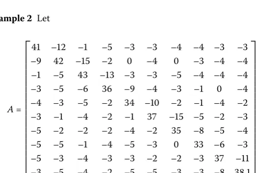
Table 2 The lower upper ofτ(A)

Method t t

Theorem 4.1 of [3] 0.10000000 Corollary 3.4 of [4] 0.12651607 Corollary 4.4 of [5] 0.15589448 Corollary 1 t= 1 0.62192050

t= 2 0.80351392

t= 3 0.90177936

t= 4 0.95648966

t= 5 0.98380481

t= 6 0.99943436

t= 7 1.00847717

t= 8 1.01247467

t= 9 1.01419855

t= 10 1.01473510

Example  Let

A= ⎡ ⎢ ⎢ ⎢ ⎢ ⎢ ⎢ ⎢ ⎢ ⎢ ⎢ ⎢ ⎢ ⎢ ⎢ ⎢ ⎢ ⎢ ⎢ ⎣

 – – – – – – – – – –  – –  –  – – – – –  – – – – – – – – – –  – – – –  – – – – –  – – – – – – – – – –  – – – – – – – – – –  – – – – – – – – –   – – – – – – – – – –  – – – – – – – – – – .

⎤ ⎥ ⎥ ⎥ ⎥ ⎥ ⎥ ⎥ ⎥ ⎥ ⎥ ⎥ ⎥ ⎥ ⎥ ⎥ ⎥ ⎥ ⎥ ⎦ .

SinceA∈Znis strictly row diagonally dominant, it is easy to see thatAis a

nonsingu-larM-matrix. Numerical results obtained from Theorem . of [], Corollary . of [], Corollary . of [], and Corollary ,i.e., inequalities (), (), (), and (), respectively, are given in Table  for the total number of iterationsT= . In fact,τ(A) = ..

Remark  Numerical results in Table  and Table  show that:

(a) Lower bounds obtained from Theorem  and Corollary  are bigger than these corresponding bounds in [–].

(b) These sequences obtained from Theorem  and Corollary  are monotone increasing.

(c) These sequences obtained from Theorem  and Corollary  approximates eﬀectively the true value ofτ(A).

Example  LetA= [aij]∈R×, whereaii= ,i∈N;aij= –,i,j∈N,i=j. It is easy to

know thatAis a nonsingularM-matrix andA–is doubly stochastic. By Theorem  for T= , we haveτ(A)≥ whent= . In fact,τ(A) = .

(9)

4 Further work

In this paper, we present several convergent sequences to approximateτ(A). Then an in-teresting problem is how accurately these bounds can be computed. At present, it is very diﬃcult for the authors to give the error analysis. We will continue to study this problem in the future.

Competing interests

The authors declare that they have no competing interests.

Authors’ contributions

All authors contributed equally to this work. All authors read and approved the ﬁnal manuscript.

Acknowledgements

This work is supported by the National Natural Science Foundation of China (Nos. 11361074, 11501141), Foundation of Guizhou Science and Technology Department (Grant No. [2015]2073), Scientiﬁc Research Foundation for the introduction of talents of Guizhou Minzu University (No. 15XRY003), and Scientiﬁc Research Foundation of Guizhou Minzu University (No. 15XJS009).

Received: 12 January 2016 Accepted: 6 April 2016

References

1. Berman, A, Plemmons, RJ: Nonnegative Matrices in the Mathematical Sciences. SIAM, Philadelphia (1994) 2. Horn, RA, Johnson, CR: Topics in Matrix Analysis. Cambridge University Press, Cambridge (1991)

3. Shivakumar, PN, Williams, JJ, Ye, Q, Marinov, CA: On two-sided bounds related to weakly diagonally dominant

M-matrices with application to digital circuit dynamics. SIAM J. Matrix Anal. Appl.17, 298-312 (1996)

4. Tian, GX, Huang, TZ: Inequalities for the minimum eigenvalue ofM-matrices. Electron. J. Linear Algebra20, 291-302 (2010)

5. Li, CQ, Li, YT, Zhao, RJ: New inequalities for the minimum eigenvalue ofM-matrices. Linear Multilinear Algebra61(9), 1267-1279 (2013)

6. Wang, F, Sun, DF: Some new inequalities for the minimum eigenvalue ofM-matrices. J. Inequal. Appl.2015, 195 (2015) 7. Zhao, JX, Wang, F, Sang, CL: Some inequalities for the minimum eigenvalue of the Hadamard product of anM-matrix

and an inverseM-matrix. J. Inequal. Appl.2015, 92 (2015)

8. Zhou, DM, Chen, GL, Wu, GX, Zhang, XY: On some new bounds for eigenvalues of the Hadamard product and the Fan product of matrices. Linear Algebra Appl.438, 1415-1426 (2013)

9. Zhou, DM, Chen, GL, Wu, GX, Zhang, XY: Some inequalities for the Hadamard product of anM-matrix and an inverse