R E S E A R C H
Open Access
LQP method with a new optimal step size
rule for nonlinear complementarity problems
Ali Ou-yassine
1, Abdellah Bnouhachem
1,2*and Fatimazahra Benssi
1*Correspondence:
[email protected] 1Laboratoire d’Ingénierie des
Systémes et Technologies de l’Information, ENSA, Ibn Zohr University, Agadir, BP 1136, Morocco 2School of Management Science
and Engineering, Nanjing University, Nanjing, 210093, P.R. China
Abstract
Inspired and motivated by results of Bnouhachemet al.(Hacet. J. Math. Stat. 41(1):103-117, 2012), we propose a new modified LQP method by using a new optimal step size, where the underlying functionFis co-coercive. Under some mild conditions, we show that the method is globally convergent. Some preliminary computational results are given to illustrate the efficiency of the proposed method.
Keywords: nonlinear complementarity problems; co-coercive operator; logarithmic-quadratic proximal method
1 Introduction
The nonlinear complementarity problem (NCP) is to determine a vectorx∈Rnsuch that
x≥, F(x)≥ and xTF(x) = , (.)
whereFis a nonlinear mapping fromRninto itself. Complementarity problems introduced
by Lemke [] and Cottle and Dantzig [] in the early s has attracted great attention of
researchers (see,e.g., [, ] and the references therein). On the one hand, there have been
many theoretical results on the existence of solutions and their structural properties. On the other hand, many attempts have been made to develop implementable algorithms for the solution of NCP. A popular way to solve the NCP is to reformulate as finding the zero
point of the operatorT(x) =F(x) +NRn
+(x),i.e., findx
∗∈Rn
+such that ∈T(x∗), where
NRn+(·) is the normal cone operator toR
n
+defined by
NRn+(x) =
{y∈Rn:yT(v–x)≤,∀v∈Rn
+} ifx∈Rn+,
∅ otherwise.
The proximal point algorithm (PPA) is recognized as a powerful and successful algorithm in finding a solution of maximal monotone operators, and it has been proposed by
Mar-tinet [] and studied by Rockafellar []. Starting from any initialx∈Rnand for positive
realβk≥β> , iteratively updatingxk+conforming to the following problem:
∈βkT(x) +∇xqx,xk, (.)
where
qx,xk=
x–x
k
, (.)
is a quadratic function ofx. In place of the usual quadratic term many researchers have
used some nonlinear functionsr(x,xk); see, for example, [–]. Auslenderet al.[, ]
proposed a new type of proximal interior method through replacing the second term of (.) by
x– ( –μ)xk–μXkx– (.)
or
x–xk+μXklog
x xk
, (.)
whereμ∈(, ) is a given constant,Xk=diag(xk
,xk, . . . ,xkn), andx–is ann-vector whose
jth elements isx
j. It is easy to see that, at thekth iteration, solving (.) by the LQP method
is equivalent to the following system of nonlinear equations:
βkF(x) +x– ( –μ)xk–μXkx–= (.)
or
βkF(x) +x–xk+μXklog
x xk
= . (.)
Solving the subproblem (.) or (.) exactly is typically hard demand in practice. To
over-come this difficulty, Heet al.[], Bnouhachem [, ], Bnouhachem and Yuan [],
Bnouhachem and Noor [, ], Bnouhachemet al.[, ], Noor and Bnouhachem [],
and Xuet al.[] introduced some LQP-based prediction-correction methods which do
not suffer from the above difficulty and make the LQP method more practical. Each itera-tion of the above methods contain a predicitera-tion and a correcitera-tion, the predictor is obtained via solving the LQP system approximately under significantly relaxed accuracy criterion and the new iterate is computed directly by an explicit formula derived from the original LQP method for [], while the new iterate is computed by using the projection operator for [, , ]. Inspired and motivated by the above research, we suggest and analyze a new LQP method for solving nonlinear complementarity problems (.) by using a new
step sizeαkto Bnouhachem’s LQP method []. We also study the global convergence of
the proposed modified LQP method under some mild conditions.
Throughout this paper we assume that F is co-coercive with modulus c> , that is,
F(x) –F(y),x–y ≥cF(x) –F(y),∀x,y∈Rn+and the solution set of (.), denoted by∗, is nonempty.
2 The proposed method and some properties
In this section, we suggest and analyze the new modified LQP method for solving NCP
(.). For givenxk> andβk> , each iteration of the proposed method consists of two
Prediction step: Find an approximate solutionx˜kof (.), called predictor, such that
≈βkFx˜k+x˜k– ( –μ)xk–μXkx˜k–=ξk:=βk
Fx˜k–Fxk (.)
andξkwhich satisfies
ξk≤ηxk–x˜k, <η< . (.)
Correction step: For <ρ< , the new iteratexk+(αk) is defined by
xk+(αk) =ρxk+ ( –ρ)PRn+
xk–αkd
xk,βk , (.)
where
dxk,βk
:=xk–x˜k+ βk
+μF
˜
xk (.)
andαkis a positive scalar. How to choose a suitableαkwe will discuss later.
Remark . Equation (.) can be written as
βkF
xk+x˜k– ( –μ)xk–μXkx˜k–= , (.)
and the solution of (.) can be componentwise obtained by
˜
xkj =
( –μ)xkj –βkFj(xk) +[( –μ)xk
j –βkFj(xk)]+ μ(xkj)
. (.)
Moreover, for anyxk> we have alwaysx˜k> .
We now consider the criterion forαk, which ensures thatxk+(αk) is closer to the solution
set thanxk. For this purpose, we define
(αk) =xk–x∗
–xk+(αk) –x∗
. (.)
Theorem .[] Let x∗∈∗,xk+(α
k)be defined by(.),then we have
(αk)≥( –ρ)
αk
xk–x˜kTDxk,βk
–αkDxk,βk
+ Dxk,βk T
xk–x˜k
+
αk
+μ
–μ–βk
c
–αkxk–x˜k
, (.)
where
Dxk,βk
:=xk–x˜k+
+μξ
Lemma .[] For given xk∈Rn
++,let x˜k satisfy the condition(.), then we have the following:
xk–x˜kTDxk,βk
≥
–η
+μ
xk–x˜k (.)
and
xk–x˜kTDxk,βk
≥
D
xk,βk. (.)
From (.), we have
(αk)≥( –ρ)
αk
xk–x˜kTDxk,βk
–αkDxk,βk
+ Dxk,βk T
xk–x˜k
+
αk
+μ
–μ–βk
c
–αkxk–x˜k
= ( –ρ)
αk
xk–x˜kTDxk,βk
+
+μ
–μ–βk
c
xk–x˜k
–αkDxk,βk+ D
xk,βk T
xk–x˜k+xk–x˜k
= ( –ρ)
αk
xk–x˜kTDxk,βk
+
+μ
–μ–βk
c
xk–x˜k
–αkDxk,βk
+xk–x˜k
= ( –ρ) (αk), (.)
where
(αk) := αk
xk–x˜kTDxk,βk
+
+μ
–μ–βk
c
xk–x˜k
–αkDxk,βk
+xk–x˜k. (.)
3 Convergence analysis
In this section, we prove some useful results which will be used in the consequent analysis
and then investigate the strategy of how to choose the new step sizeαk.
Note that (αk) is a quadratic function ofαkand it reaches its maximum at
α∗k=(x
k–x˜k)TD(xk,β
k) ++μ( –μ– βk c)x
k–x˜k
D(xk,β
k) +xk–x˜k
(.)
and
α∗k=αk∗xk–x˜kTDxk,β k
+
+μ
–μ–βk
c
xk–x˜k
. (.)
In the next theorem we show thatαk∗and (αk∗) are lower bounded away from zero,
Theorem . For given xk∈Rn
++,letx˜ksatisfy the condition(.)andβksatisfy
<βl≤ ∞ inf k=βk≤
∞ sup
k=
βk≤βu< c( –μ),
then we have the following:
α∗k≥ –η
– η+μ> (.)
and
α∗k≥ ( –η)
( – η+μ)( +μ)x
k–x˜k. (.)
Proof It follows from (.) and (.) that
α∗k = (x
k–x˜k)TD(xk,β
k) ++μ( –μ– βk c)x
k–x˜k
D(xk,β
k) +xk–x˜k
≥ (xk–x˜k)TD(xk,βk)
D(xk,β
k) +xk–x˜k
= (x
k–x˜k)TD(xk,β k)
D(xk,β
k)+ D(xk,βk)T(xk–x˜k) +xk–x˜k
≥ (xk–x˜k)TD(xk,βk)
( ++–μη)D(xk,β
k)T(xk–x˜k)
= –η
– η+μ> .
Using (.), (.), and (.), we have
α∗k≥
–η
– η+μ
–η
+μ+
+μ
–μ–βk
c
xk–x˜k
≥ ( –η)
( – η+μ)( +μ)x
k–x˜k.
Remark . Note thatαk∗
=min{( –μ–
βk
c)/( +μ),
(xk–˜xk)TD(xk,βk) D(xk,β
k)+D(xk,βk)T(xk–˜xk)}
is the
op-timal step size used in []. Sinceαk∗is to maximize the profit function (αk), we have
α∗k≥ αk∗. (.)
Inequality (.) shows theoretically that the proposed method is expected to make more progress than that in [] at each iteration, and so it explains theoretically that the pro-posed method outperforms the method in [].
For fast convergence, we take a relaxation factorγ ∈[, ) and set the step sizeαkin (.)
byαk=γ α∗k, it follows from (.), (.), and Theorem . that
(αk)≥γ( –γ)( –ρ)
α∗k
≥γ( –γ)( –ρ) ( –η)
( – η+μ)( +μ)x
k–x˜k
Then from definition of(αk) and (.) there is a constant
τ:=γ( –γ)( –ρ) ( –η)
( – η+μ)( +μ)>
such that
xk+(αk) –x∗
≤xk–x∗–τxk–x˜k, ∀x∗∈∗. (.)
The following result can be proved by similar arguments to those in [, , , ]. Hence the proof will be omitted.
Theorem .[, , , ] Ifinf∞k=βk=βl> ,then the sequence{xk}generated by the
proposed method converges to some x∞which is a solution of NCP.
The detailed algorithm is as follows.
Step . Letβ= ,η(:= .) < , <ρ< , <μ< ,γ= .,= –,k= , andx> .
Step . Ifmin(x,F(x))∞≤, then stop. Otherwise, go to Step . Step . (Prediction step)
s:= ( –μ)xk–βkFxk, x˜ki :=si+
(si)+ μxk i
/,
ξk:=βk
Fx˜k–Fxk, r:=ξk/xk–x˜k
while(r>η)
βk:=βk∗./r,
s:= ( –μ)xk–βkFxk, x˜ki :=
si+
(si)+ μxk i
/,
ξk:=βk
Fx˜k–Fxk, r:=ξk/xk–x˜k.
end while
Step . (Correction step)
Dxk,βk
:=xk–x˜k+
+μξ
k, dxk,β k
:=xk–x˜k+ βk
+μF
˜
xk,
α∗k=(x
k–x˜k)TD(xk,β
k) ++μ( –μ–βkc)xk–x˜k
D(xk,β
k) +xk–x˜k
, αk=γ αk∗,
xk+=ρxk+ ( –ρ)PRn
+
xk–αkdxk,βk .
Step .
βk+= β
k∗.
r , ifr≤.;
βk, otherwise.
4 Preliminary computational results
In this section, we consider two examples to illustrate the efficiency and the performance of the proposed algorithm.
4.1 Numerical experiments I
We consider the nonlinear complementarity problems
x≥, F(x)≥, xTF(x) = , (.)
where
F(x) =D(x) +Mx+q,
D(x) andMx+qare the nonlinear part and linear part ofF(x), respectively.
We form the linear part in the test problems similarly to Harker and Pang []. The matrix
M=ATA+B, whereAis ann×nmatrix whose entries are randomly generated in the
interval (–, +) and a skew-symmetric matrixBis generated in the same way. The vector
qis generated from a uniform distribution in the interval (–, ) or in (–, ). In
D(x), the nonlinear part ofF(x), the components are chosen to beDj(x) =dj∗arctan(xj),
wheredjis a random variable in (, ).
In all tests we take the logarithmic proximal parameterμ= .,ρ= ., andc= .. All
iterations start withx= (, . . . , )Tandβ
= , and we have the stopping criterion
when-ever
minxk,Fxk∞≤–.
All codes were written in Matlab, and we compare the proposed method with that in
[]. The test results for problem (.) are reported in Tables and .kis the number of
iteration andldenotes the number of evaluations of mappingF.
Tables and show that the proposed method is more efficient. Numerical results
in-dicate that the proposed method can be save about ∼ percent of the number of
iterations and about ∼ of the amount of computing the value of functionF.
4.2 Numerical experiments II
In this subsection, we apply the proposed method to the traffic equilibrium problems and present corresponding numerical results.
Consider a network [N,L] of nodes Nand directed links L, which consists of a finite
[image:7.595.189.404.641.732.2]sequence of connecting links with a certain orientation. Leta,b,etc.denote the links, and
Table 1 Numerical results for problem (4.1) withq∈(–500, 500)
n The method in [18] The proposed method
k l CPU (Sec.) k l CPU (Sec.)
200 297 651 0.068 117 279 0.016
300 329 708 0.094 129 310 0.029
400 333 721 0.13 169 367 0.08
500 368 801 0.22 171 381 0.12
700 364 751 0.41 142 334 0.12
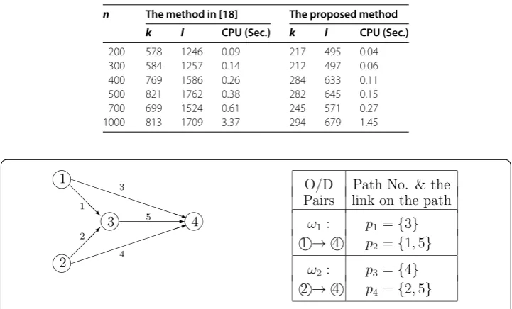
Table 2 Numerical results for problem (4.1) withq∈(–500, 0)
n The method in [18] The proposed method
k l CPU (Sec.) k l CPU (Sec.)
200 578 1246 0.09 217 495 0.04
300 584 1257 0.14 212 497 0.06
400 769 1586 0.26 284 633 0.11
500 821 1762 0.38 282 645 0.15
700 699 1524 0.61 245 571 0.27
1000 813 1709 3.37 294 679 1.45
Figure 1 An illustrative example of given directed network and the O/D pairs.
letp,q,etc.denote the paths. We letωdenote an origin/destination (O/D) pair of nodes
of the network andPωdenotes the set of all paths connecting O/D pairω. Note that the
path-arc incidence matrix and the path-O/D pair incidence matrix, denoted byAandB,
respectively, are determined by the given network and O/D pairs. To see how to convert a traffic equilibrium problem into a variational inequality, we take into account a simple example as depicted in Figure .
For the given example in Figure , the path-arc incidence matrixAand the path-O/D
pair incidence matrixBhave the following forms:
No. link
A=
⎛ ⎜ ⎜ ⎜ ⎝
⎞ ⎟ ⎟ ⎟ ⎠,
No. O/Dpair ω ω
B=
⎛ ⎜ ⎜ ⎜ ⎝
⎞ ⎟ ⎟ ⎟ ⎠.
Letxprepresent the traffic flow on pathpandfadenote the link load on linka, then the
arc-flow vectorf is given by
f =ATx.
Letdωdenote the traffic amount between O/D pairω, which must satisfy
dω=
p∈Pω
xp.
Thus, the O/D pair-traffic amount vectordis given by
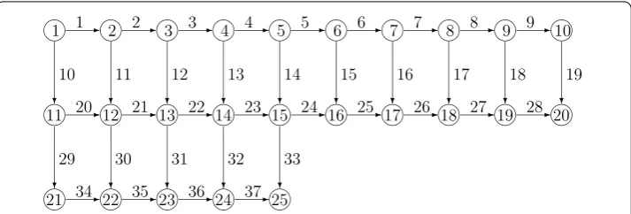
[image:8.595.142.386.481.555.2]Figure 2 A directed network with 25 nodes and 37 links.
Lett(f) ={ta,a∈L}be the vector of link travel costs, which is a function of the link flow.
A user traveling on pathpincurs a (path) travel costθp. For given link travel cost vectort,
the path travel cost vectorθis given by
θ=At(f) and thus θ(x) =AtATx.
Associated with every O/D pairω, there is a travel disutilityλω(d). Since both the path
costs and the travel disutilities are functions of the flow patternx, the traffic network
equi-librium problem is to seek the path flow patternx∗such that
x∗≥, x–x∗TFx∗≥, ∀x≥, (.)
where
Fp(x) =θp(x) –λω
d(x), ∀ω,p∈Pω,
and thus
F(x) =AtATx–BλBTx.
We apply the proposed method to the example taken from [] (Example . in []), which consisted of nodes, links and six O/D pairs. The network is depicted in Fig-ure .
For this example, there are together paths for the six given O/D pairs and hence the
dimension of the variablexis . Therefore, the path-arc incidence matrixAis a ×
matrix and the path-O/D pair incidence matrixBis a × matrix. The user cost of
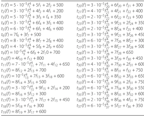
traversing linkais given in Table . The disutility function is given by
λω(d) = –mωdω+qω (.)
and the coefficientsmω andqωin the disutility function of different O/D pairs for this
example are given in Table .
The test results for problems (.) for differentεare reported in Table ,kis the number
Table 3 The link traversing cost functionsta(f) in the example
[image:10.595.170.424.325.381.2]t1(f) = 5·10–5f14+ 5f1+ 2f2+ 500 t20(f) = 3·10–5f204 + 6f20+f21+ 300 t2(f) = 3·10–5f24+ 4f2+ 4f1+ 200 t21(f) = 4·10–5f214 + 4f21+f22+ 400 t3(f) = 5·10–5f34+ 3f3+f4+ 350 t22(f) = 2·10–5f224 + 6f22+f23+ 500 t4(f) = 3·10–5f44+ 6f4+ 3f5+ 400 t23(f) = 3·10–5f234 + 9f23+ 2f24+ 350 t5(f) = 6·10–5f54+ 6f5+ 4f6+ 600 t24(f) = 2·10–5f244 + 8f24+f25+ 400 t6(f) = 7f6+ 3f7+ 500 t25(f) = 3·10–5f254 + 9f25+ 3f26+ 450 t7(f) = 8·10–5f74+ 8f7+ 2f8+ 400 t26(f) = 6·10–5f264 + 7f26+ 8f27+ 300 t8(f) = 4·10–5f84+ 5f8+ 2f9+ 650 t27(f) = 3·10–5f274 + 8f27+ 3f28+ 500 t9(f) = 10–5f94+ 6f9+ 2f10 + 700 t28(f) = 3·10–5f284 + 7f28+ 650 t10(f) = 4f10+f12+ 800 t29(f) = 3·10–5f294 + 3f29+f30+ 450 t11(f) = 7·10–5f114 + 7f11+ 4f12+ 650 t30(f) = 4·10–5f304 + 7f30+ 2f31+ 600 t12(f) = 8f12+ 2f13+ 700 t31(f) = 3·10–5f314 + 8f31+f32+ 750 t13(f) = 10–5f134 + 7f13+ 3f18+ 600 t32(f) = 6·10–5f324 + 8f32+ 3f33+ 650 t14(f) = 8f14+ 3f15+ 500 t33(f) = 4·10–5f334 + 9f33+ 2f31+ 750 t15(f) = 3·10–5f154 + 9f15+ 2f14+ 200 t34(f) = 6·10–5f344 + 7f34+ 3f30+ 550 t16(f) = 8f16+ 5f12+ 300 t35(f) = 3·10–5f354 + 8f35+ 3f32+ 600 t17(f) = 3·10–5f174 + 7f17+ 2f15+ 450 t36(f) = 2·10–5f364 + 8f36+ 4f31+ 750 t18(f) = 5f18+f16+ 300 t37(f) = 6·10–5f374 + 5f37+f36+ 350 t19(f) = 8f19+ 3f17+ 600
Table 4 The O/D pairs and the parameters in (4.3) of the example
(O,D) Pairω (1, 20) (1, 25) (2, 20) (3, 25) (1, 24) (11, 25)
mω 1 6 10 5 7 9
qω 1,000 800 2,000 6,000 8,000 7,000
[image:10.595.190.406.410.494.2]|Pω| 10 15 9 6 10 5
Table 5 Numerical results for differentε
Differentε The method in [18] The proposed method
k l CPU (Sec.) k l CPU (Sec.)
10–5 201 445 0.04 90 216 0.11
10–6 263 580 0.034 115 276 0.01
10–7 321 708 0.054 150 352 0.019
10–8 380 837 0.058 183 426 0.018
10–9 438 963 0.061 211 491 0.02
is
min{x,F(x)}∞
min{x,F(x)}∞ ≤ε.
Table shows that the new method is more flexible and efficient to solve a traffic equilib-rium problem. Moreover, it demonstrates computationally that the new method is more effective than the method presented in [] in the sense that the new method needs fewer
iteration and less evaluation numbers ofF, which clearly illustrates its efficiency.
Competing interests
The authors declare that they have no competing interests.
Authors’ contributions
All authors have made equal contributions. All authors read and approved the final manuscript.
Acknowledgements
Received: 20 April 2015 Accepted: 12 June 2015 References
1. Lemke, CE: Bimatrix equilibrium point and mathematical programming. Manag. Sci.11, 681-689 (1965) 2. Cottle, RW, Dantzig, GB: Complementary pivot theory of mathematical programming. Linear Algebra Appl.1,
103-125 (1968)
3. Ferris, MC, Pang, JS: Engineering and economic applications of complementary problems. SIAM Rev.39, 669-713 (1997)
4. Harker, PT, Pang, JS: Finite-dimensional variational inequality and nonlinear complementarity problems: a survey of theory, algorithms and applications. Math. Program.48, 161-220 (1990)
5. Martinet, B: Determination approchée d’un point fixe d’une application pseudo-contractante. C. R. Acad. Sci. Paris
274, 163-165 (1972)
6. Rockafellar, RT: Monotone operators and the proximal point algorithm. SIAM J. Control Optim.14, 877-898 (1976) 7. Eckestein, J: Approximate iterations in Bregman-function-based proximal algorithms. Math. Program.83, 113-123
(1998)
8. Guler, O: On the convergence of the proximal point algorithm for convex minimization. SIAM J. Control Optim.29, 403-419 (1991)
9. Teboulle, M: Convergence of proximal-like algorithms. SIAM J. Optim.7, 1069-1083 (1997)
10. Auslender, A, Teboulle, M, Ben-Tiba, S: A logarithmic-quadratic proximal method for variational inequalities. Comput. Optim. Appl.12, 31-40 (1999)
11. Auslender, A, Teboulle, M, Ben-Tiba, S: Interior proximal and multiplier methods based on second order homogenous Kernels. Math. Oper. Res.24, 646-668 (1999)
12. He, BS, Liao, LZ, Yuan, XM: A LQP based interior prediction-correction method for nonlinear complementarity problems. J. Comput. Math.24(1), 33-44 (2006)
13. Bnouhachem, A: A new inexactness criterion for approximate logarithmic-quadratic proximal methods. Numer. Math., Theory Methods Appl.15(1), 74-81 (2006)
14. Bnouhachem, A: An LQP method for pseudomonotone variational inequalities. J. Glob. Optim.36(3), 351-363 (2006) 15. Bnouhachem, A, Yuan, XM: An extended LQP method for monotone nonlinear complementarity problems. J. Optim.
Theory Appl.135(3), 343-353 (2007)
16. Bnouhachem, A, Noor, MA: A new predictor-corrector method for pseudomonotone nonlinear complementarity problems. Int. J. Comput. Math.85, 1023-1038 (2008)
17. Bnouhachem, A, Noor, MA: An interior proximal point algorithm for nonlinear complementarity problems. Nonlinear Anal. Hybrid Syst.4(3), 371-380 (2010)
18. Bnouhachem, A, Noor, MA, Khalfaoui, M, Zhaohan, S: An approximate proximal point algorithm for nonlinear complementarity problems. Hacet. J. Math. Stat.41(1), 103-117 (2012)
19. Bnouhachem, A, Noor, MA, Khalfaoui, M, Zhaohan, S: A new logarithmic-quadratic proximal method for nonlinear complementarity problems. Appl. Math. Comput.215, 695-706 (2009)
20. Noor, MA, Bnouhachem, A: Modified proximal point methods for nonlinear complementarity problems. J. Comput. Appl. Math.197, 395-405 (2006)
21. Xu, Y, He, BS, Yuan, X: A hybrid inexact logarithmic-quadratic proximal method for nonlinear complementarity problems. J. Math. Anal. Appl.322, 276-287 (2006)