MODELLING SRI LANKAN OIL DEMAND: AN ECONOMETRIC APPROACH

MODELLING SRI LANKAN OIL DEMAND: AN ECONOMETRIC APPROACH

M.A.H.C Munasinghe1, T.M.J.A. Cooray2

1

Lecturer, School of Computing, NSBM Green University, Sri Lanka

2

Senior Lecturer, Department of Mathematics, University of Moratuwa, Sri Lanaka Contact Person: Ms. M. A. H.C Munasinghe/ [email protected]

ABSTRACT

This study examines the effect of economic variables, Goss Domestic Product (GDP),

Foreign Direct Investment (FDI), Population and Oil Price on oil consumption in Sri Lanka

using an Error Correction Model. Yearly data of oil consumption, Goss Domestic Product

(GDP), Foreign Direct Investment (FDI), Sri Lankan population and crude oil price during

the period 1988 – 2013 were used in the analysis. All the data have been obtained by the

online data sources of World Bank and United States energy information administration. This

research involves estimating the elasticity of Goss Domestic Product (GDP), Foreign Direct

Investment (FDI), Sri Lankan population and crude oil price on crude oil consumption in Sri

Lanka.

Unit root test confirmed that series are not stationary in its levels but they are stationary in

first difference. Therefore the study uses the Engle-Ganger cointegation method to create a

dynamic short run model. Also Chow - break point test was used to test the significance of a

structural break down in the data set and the dummy variable was significant in allowing for

the structural change.

The Vector Error Correction (VEC) model finds that Goss Domestic Product (GDP), Foreign

Direct Investment (FDI), population and oil price are determinants of the oil demand. It

shows that in the long run only FDI increases the overall oil demand while GDP and

population increase the oil demand in the short run.

By using the selected model, oil demand was forecasted and the Mean Absolute Percentage

Error (MAPE) of the fitted model was found less than 5 percent. Therefore the fitted model is

recommended as the suitable model to forecast oil demand. As the crude oil storage is a

common problem in Sri Lanka, forecasting oil demand can be used to find the solutions for

the challenges in the petroleum sector.

Key words: Crude oil, Demand, Determinants, Petroleum Sector, Sri Lanka

International Research Journal of Natural and Applied Sciences

ISSN: (2349-4077)

Impact Factor 5.46 Volume 6, Issue 5, May 2019

1.Introduction

Crude oil is considered as an unrefined oil product composed of organic compound which

consists of different organic materials. Crude oil is used to refine usable products like

hydrocarbon, solvents, gasoline, kerosene, diesel and various kinds of petrochemicals. It is an

unrenewable resource, which implies that it cannot be replaced naturally at the speed of

consumption. Hence it is considered as a limited resource.

Global crude oil demand is around 90 million barrels per day (Mbd), from that 50% is

consumed by the countries who are members of Organization for Economic Corporation and

Development (OECD) [16]. Sri Lanka’s crude oil consumption is very small compared with

the world demand. Sri Lanka has been an importer of crude oil for a long time and the country

spends 24% of the import price on it. The Ceylon Petroleum Corporation (CPC) has been a

monopoly supplier of fossil oil to the native market. However, Lanka Indian Oil Corporation

(LIOC) was added to the market to form a duopoly within the fossil oil product distribution in

2003.

Sri Lanka is importing refined products since many years for domestic consumption. Hence

the demand of the petroleum products are increasing in both volume and value terms. CPC

was ready to meet the overall fossil oil product demand of the country through its solely plant

within the nineteen seventies. As the emerging need of crude oil demand, now Sri Lanka depends on foreign refined product sources because the provide capability of the CPC’s plant

remained as a constant. In 2011 local petroleum demand was 4200 million (Mn) liters per

year and from that only one third is provided by local refined imported crude oil. The

remaining amount is imported as refined products. Consequently the country is spending a

large amount of money for importing crude oil products. From 2009- 2011 the petroleum bill

has more than doubled. If the trend keeps on continuing like this we have to arrange a

considerable proportion of resources to import crude oil.

Currently Sri Lanka is facing for several challenges in petroleum industry. Among them

uncertainty of supply due to current tension in the middle east and diversification of the

resources due to technological issues are main concerns. The recent crude oil crisis in Sri

Lanka is also attributed to the limited supply of crude oil. Although we have a duopoly market

for crude oil in Sri Lanka, both are import dependent to a lager extent. Hence the challenges

As in 2011 petroleum accounts for 24% of import bill and 45% of exports. Hence more

resources will be required for imports in absolute and relative terms in future (Samaratunga,

2014).

As it is an emerging need to get an idea about the future crude oil demand and also its

determinants, the objective of this study is to explore several important factors that cause for

Sri Lankan crude oil demand. Also this study aims to forecast the crude oil demand using a

suitable model. Hence this thesis comprises a long run and short run models using data from

1988 – 2013. This will have significant policy implications on planning the future Sri Lankan

economy and oil demand in Sri Lanka.

2. Materials and methods 2.1 Data Description

In this study Goss Domestic Product (GDP), Foreign Direct Investment (FDI), Sri Lankan

population and crude oil price were used to find out the effect on Sri Lankan oil demand.

Since problems can occur in the interpretation of variables when they are different units, the

log form of the variables have been used for this study.

The oil demand was measured by the consumption of crude oil. The stationary condition of

the first difference series was checked using the Augmented - Dickey Fuller test.

Chow - break point test was used to test the significance of a structural break down in the

data set. Hence a dummy variable was used to indicate the structural break down.

Cointegration was checked with the use of Trace statistic test. The Vector Error Correction

Methodology was used to find a model for Sri Lankan crude oil consumption.

Then the stationary condition of the error term of the Vector Error Correction Model was

checked using the Augmented - Dickey Fuller unit root test and a residual analysis was

carried out to check the validity of the model. Stability of the coefficients of the model is

checked by Cusum test. Impulse response function was used to study the dynamic effects of

shocks of macroeconomic variables on oil demand. Variance decomposition method was

used to evaluate dynamic interactions and strength of casual relations among variables in the

system.

All the data have been collected using online resources of World Bank and United States

Energy Information Administration. The sample period for this study is 1988 through 2013.

The software employed in this research is EViews 8.0. The description of variables used in

this research study is given below.

LNCON – Log of Oil Consumption in Sri Lanka

LNFDI –Log ofForeign Direct Investment (FDI)

LNPOP –Log of Sri Lankan Population

LNOILPRICE –Log ofCrude Oil Price

2.2 Stationary Test

The most widely used test to check the stationary condition is the unit root test. The presence

of unit root indicates that the data series is non stationary. There are two standard procedures

of unit root test namely the Augmented Dickey Fuller (ADF) test and Phillips-Perron (PP)

test. This study has used the Augmented Dickey Fuller (ADF) test to check the stationary

condition of the series.

2.2 Vector Error Correction Modeland Cointegration Test

Engle and Granger (1987) point out that a linear combination of two or more non stationary

series may be stationary. The stationary combination may be interpreted as the cointegration,

or equilibrium relationship between the variables

A Vector Error CorrectionModel (VECM) is a restricted Vector Auto Regression (VAR)

model. The Vector Error Correction specification restricts the long run behavior of the

endogenous variables to converge to their long run equilibrium relationships and allow the

short run dynamics.

The VAR model is a general framework used to describe the dynamic interrelationship

among stationary variables. So, the first step in time-series analysis should be to determine

whether the levels of the data are stationary. If not, take the first differences of the series and

should try again. Usually, if the levels of the time series data are not stationary, the first

differences will be.

If the time series are not stationary then the VAR framework needs to be modified to allow

consistent estimate of the relationships among the series. The Vector Error Correction (VEC)

model is just a special case of the VAR for variables that are stationary in their differences

(i.e. I(1)). The Vector Error Correction Model can also take into account any cointegrating

relationships among the variables.

Suppose 𝑥𝑡 and 𝑦𝑡 are I(1) and cointegrated. Then ∈𝑡is I(0) in the cointegrating equation 𝑦𝑡 = 𝛼 + 𝛽𝑥𝑡 +∈𝑡

estimating an error correction model, which contains first differences of 𝑥_𝑡 and 𝑦_𝑡 , their lags,

and an error correction term. An Error Correction Model is

∆𝑦_𝑡 = 𝜇 + 𝛾₁∆𝑦_𝑡−1 + ⋯ + 𝛾_𝑝∆𝑦_𝑡−𝑝+ 𝜔₁∆𝑥_𝑡−1+ ⋯ + 𝜔_𝑟∆𝑥_𝑡−𝑟+ 𝜆𝐸𝐶_𝑡−1+ 𝑢_𝑡

where 𝜇, 𝛾_𝑖, 𝜔_𝑗, 𝜆 are the parameters of the model and 𝐸𝐶_𝑡−1 = 𝑦_𝑡− (𝑎 + 𝑏𝑥_𝑡), the error correction term, is the lagged OLS residual from the cointegrating equation. Normally 𝜆 is

expected to be negative. Then 𝜆𝐸𝐶_𝑡−1 represents a force pulling 𝑦_𝑡 toward its long-run relationship, being negative when 𝐸𝐶_𝑡−1 > 0, and positive when 𝐸𝐶_𝑡−1 < 0. 𝑢_𝑡 is the random

error. The cointegrating equation and ECM can be shown to follow from a single dynamic regression model in levels when 𝑦_𝑡 and𝑥_𝑡 are cointegrated.

To capture the cointegration the trace test was used. The trace test examines the number of

linear combinations (i.e. K) to be equal to a given value 𝐾₀ (where𝐾₀ = 0,1,2 … ) , and the alternative hypothesis for K to be greater than 𝐾₀

𝐻0: 𝐾 = 𝐾0 𝐻₀: 𝐾 > 𝐾₀

To test for the existence of cointegration using the trace test, we set 𝐾₀ = 0 (no

cointegration), and examine whether the null hypothesiscan be rejected. If this is the case,

then we conclude there is at least one cointegration relationship.

In this case, we need to reject the null hypothesis to establish the presence of cointegration

between the variables.

2.3 Impulse Response Function and Variance Decomposition

Since the cointegration analysis only captures the long run relationship among the variables,

Impulse Response Function and Variance Decomposition method were used to find how the

oil demand responds to shocks in the macroeconomic variables.

2.4 ARCH Test for Heteroscedasticity

Engle’s ARCH test is used to test the Heteroscedasticity among the residuals of a given

model. The null hypothesis of the test is that a series of residuals (rt) exhibits no conditional

heteroscedasticity (ARCH effects), against the alternative that an ARCH(L) model describes

the series.

The ARCH(L) model has the following form:

r_t2 _{= a}

0+ a1r2t−1+⋯+aLr2t−L+et (1)

where r_t denotes the residuals andetdenotes the random error. Also ajs are parameters of the model wherethere is at least one a_j ≠ 0, j = 0 … L

The test statistic is the Lagrange multiplier statistic; TR2_~χ

L 2

where: T is the sample size and R2 is the coefficient of determination from fitting the ARCH(L) model for a number of lags (L) via regression.

Under the null hypothesis, the asymptotic distribution of the test statistic is chi-square

with L degrees of freedom.

To test the null hypothesis that there is no ARCH up to order L in the residuals, we run the

regression denoted by equation (1). Then the R2value has to be calculated and then the test statistic value can be obtained by multiplying the R2value by sample size. The null hypothesis can be rejected if the calculated value of the test statistic is greater than the chi square critical

value

2.5 LM test for Serial Correlation

This test is an alternative to the Q-statistics for testing serial correlation. The test belongs to

the class of asymptotic (large sample) tests known as Lagrange multiplier (LM) tests.

H0: No serial correlation up to lag order p, where p is a pre-specified integer. H1: There is serial correlation up to lag order p, where p is a pre-specified integer.

The test statistic for this test is computed by an auxiliary regression as follows. First, suppose

we have estimated the regression;

𝑦𝑡 = 𝛽𝑥𝑡 + 𝜖𝑡

where 𝛽 are the estimated coefficients and 𝜖_𝑡are the errors. The test statistic for lag order p is based on the auxiliary regression for the residuals 𝜖_𝑡 = 𝑦_𝑡 − 𝛽𝑥_𝑡

This is a regression of the residuals on the original regressors X and lagged residuals upto

order p. To test the hypothesis we use the Breusch-Godfrey LM test statistic.

𝑛 ∗ 𝑅

_~𝜒

𝑑𝑓2

This is computed as the number of observations, times the R2 from theauxiliary regression. Under quite general conditions, the LM test statistic has a chi square distribution with degrees

2.6 Normality test for residuals

H0: Residuals follow a normal distribution H1: Residuals do not follow a normal distribution

The normality test of residuals is expressed as a P value. That is if the fitted model is correct

and all scatter around the model follows a Gaussian population, what is the probability of

obtaining data whose residuals deviate from a Gaussian distribution.If the P value is large,

then the residuals pass the normality test. If the P value is small, the residuals fail the

normality test and we have evidence that your data do not follow one of the assumptions of

the regression.

3. Results and discussion

This section describes the results of this research. All the data outputs and statistical tests are included in this section.

3.1 Augmented Dickey Fuller (ADF) test

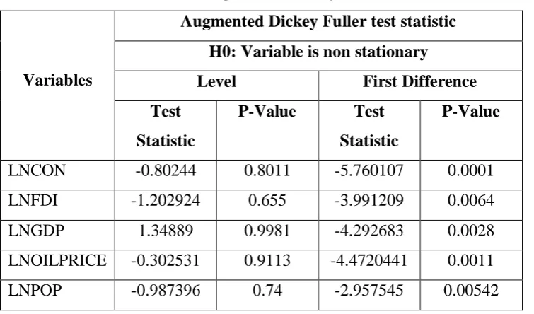
Augmented Dickey Fuller (ADF) test is used to find out whether the time series variables are

stationary. Augmented Dickey Fuller (ADF) test was performed on the examined variables at

level and also at first difference series. The Augmented Dickey Fuller (ADF) test results are

presented in table 1.

Table 1: Augmented Dickey Fuller (ADF) test results

Variables

Augmented Dickey Fuller test statistic H0: Variable is non stationary

Level First Difference

Test Statistic

P-Value Test

Statistic

P-Value

LNCON -0.80244 0.8011 -5.760107 0.0001

LNFDI -1.202924 0.655 -3.991209 0.0064

LNGDP 1.34889 0.9981 -4.292683 0.0028

LNOILPRICE -0.302531 0.9113 -4.4720441 0.0011

LNPOP -0.987396 0.74 -2.957545 0.00542

The ADF test shows that all variables are non-stationary in levels, but stationary in first

difference form. Hence we can conclude that all the variables are integrated of order one, i.e.

3.2 Chow breakpoint test to test the structural breaks

According to the results of the ADF tests all the variables are not stationary before applying

the differencing concept. Hence the Engle – Granger two step estimator was used in the

analysis.. In order to test the significance of the structural break chow breakpoint test is used.

Table 2: Chow breakpoint test using the selected variables for the model

Chow Breakpoint Test: 22

Null Hypothesis: No breaks at specified breakpoints Varying regressors: All equation variables

Equation Sample: 2 26

F-statistic 4.897459 Prob. F(5,15) 0.0074 Log likelihood ratio 24.19822 Prob. Chi-Square(5) 0.0002

As the p value of the Chow breakpoint test is less than 0.05, we reject the null hypothesis at

5% level of significance. Hence the data set contains a structural break at the 22nd data point. Therefore a dummy variable was used in the analysis.

3.3 Determining the order of lags in Vector Error Correction Model (VECM)

The number of lags to be used in the Vector Error Correction Model (VECM) should be

determined before conduct the cointegration test.

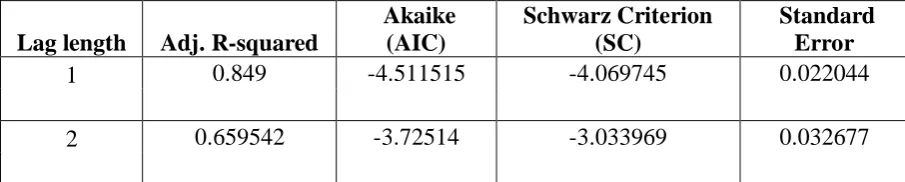
Table 3: Lag selection Criteria

Lag length Adj. R-squared

Akaike (AIC)

Schwarz Criterion (SC)

Standard Error

1 0.849 -4.511515 -4.069745 0.022044

2 0.659542 -3.72514 -3.033969 0.032677

According to table 3 lag 1 gives the values that minimize the Akaike Information Criterion,

Schwarz Criterion and Standard Error. Also lag 1 model gives the maximum value for

adjusted R squared. Hence Vector Error Correction model was fitted by considering up to lag

1 of all endogenous variables.

3.4 Cointegration Analysis

Table 4: Johansen cointegration test Date: 11/23/17 Time: 14:20

Sample (adjusted): 3 26

Included observations: 24 after adjustments Trend assumption: Linear deterministic trend

Series: LNCON LNFDI LNGDP LNPOP LNOILPRICE Lags interval (in first differences): 1 to 1

Unrestricted Cointegration Rank Test (Trace)

Hypothesized Trace 0.05

According to table1 all variables are integrated in same order. Hence Johansen cointegrated

test was used to explore the long run relationship among the variables. As for the results of

table 4, trace test indicates that there are two cointegration equations between log values of

Consumption, Gross Domestic Product (GDP), Foreign Direct Investment (FDI), Oil Price

and Population at 5% level of significance. Hence we can conclude that a Vector Error

Correction model can be used to model the relationship between these variables.

3.5 Long Run Relationship

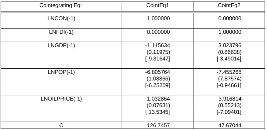
After normalization, the cointegration vectors on LNCON and normalized integrated

coefficients were estimated as reported in table 5.

Table 5: Normalized cointegration coefficients

Cointegrating Eq: CointEq1 CointEq2

LNCON(-1) 1.000000 0.000000

LNFDI(-1) 0.000000 1.000000

LNGDP(-1) -1.115634 3.023796

(0.11975) (0.86638) [-9.31647] [ 3.49014]

LNPOP(-1) -6.805764 -7.455268

(1.08856) (7.87574) [-6.25209] [-0.94661]

LNOILPRICE(-1) 1.032864 -3.916814

(0.07631) (0.55213) [ 13.5345] [-7.09401]

C 126.7457 47.67044

The first normalized equation was estimated as below:

LNCON (-1) = 126.75 + 1.03 LNOILPRICE (-1) -6.81 LNPOP (-1) -1.12 LNGDP (-1)

As it can be seen in the first normalized equation, Sri Lankan population and Gross Domestic

Product (GDP) is having a negative relationship with the oil demand in the long run while

price of oil is having a significant positive relationship with the demand of oil.

The second normalized equation was estimated as below:

LNFDI (-1) = 47.67 + 3.02LNGDP (-1) -7.46 LNPOP (-1) -3.92 LNOILPRICE (-1) None * 0.929030 127.5967 69.81889 0.0000

At most 1 * 0.805442 64.10492 47.85613 0.0008 At most 2 0.412280 24.81626 29.79707 0.1681 At most 3 0.267806 12.06014 15.49471 0.1541 At most 4 * 0.173698 4.579087 3.841466 0.0324

According to the second normalized equation, Foreign Direct Investment (FDI) is having a

significant negative relationship with the population and oil price whereas Gross Domestic

Product (GDP) is having a positive relationship with Foreign Direct Investment (FDI)

3.6 Vector Error Correction Model (VECM)

The Vector Error Correction Model (VECM) provide the correction terms that reflect the

influences of deviation of the relationship among the variables from long run equilibrium and

short run parameters. The relationship between oil demand and other macroeconomic

variables can be given in the following model. 𝑙𝑛𝑐𝑜𝑛_𝑡 =

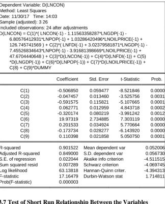
−0.1(𝑙𝑛𝑐𝑜𝑛_𝑡−1) + 0.6 𝑙𝑛𝑐𝑜𝑛_𝑡−2 + 0.13 ∗ 𝑙𝑛𝐺𝐷𝑃_𝑡−1+ 0.32 ∗ 𝑙𝑛𝐺𝐷𝑃_𝑡−2− 19.97 ∗ 𝑙𝑛𝑝𝑜𝑝𝑡−2+ 23.81 ∗ 𝑙𝑛𝑝𝑜𝑝𝑡−1 − 0.13 ∗ 𝑙𝑛𝑂𝑖𝑙𝑃𝑟𝑖𝑐𝑒𝑡−1− 0.2 ∗ 𝑙𝑛𝑂𝑖𝑙𝑃𝑟𝑖𝑐𝑒𝑡−2+ 0.01*𝑙𝑛𝐹𝐷𝐼𝑡−1− 0.06 ∗ 𝑙𝑛𝐹𝐷𝐼𝑡−2+ 67.19 − 0.11 ∗ 𝑑𝑢𝑚𝑚𝑦 The parameters of this model were estimated and shown in table 5. Table 5 consists vector

error correction model for oil demand with significant error correction terms, showing

explicit information on the long run and short run dynamic interactions. As it can be seen in

table 6 both error correction terms are significant with negative sign. This implies that long

run movements of the variables are determined by both equilibrium relationships.

According to table 6, the estimate of C(1) which is the adjustment coefficient associated with

oil demand is -0.51 and it is statistically significant. This implies that with absence of

changes in oil price, population and Gross Domestic Product (GDP), deviation of the model

from the long run path is corrected by 51% increase in LNCON annually. This means that the

deviation from the long run relationship takes approximately 2 years (1/0.51) to eliminate the

disequilibrium.

C(2) is the adjustment coefficient associated with Foreign Direct Investment (FDI). It is

-0.047 and statistically significant. This implies that with absence of changes in oil price,

population and Gross Domestic Product (GDP), deviation of the model from the long run

Table 6: Significance of the coefficients of Vector Error Correction Model (VECM) Dependent Variable: D(LNCON)

Method: Least Squares Date: 11/30/17 Time: 14:03 Sample (adjusted): 3 26

Included observations: 24 after adjustments

D(LNCON) = C(1)*( LNCON(-1) - 1.11563358287*LNGDP(-1) - 6.80576412931*LNPOP(-1) + 1.03286420496*LNOILPRICE(-1) + 126.745741569 ) + C(2)*( LNFDI(-1) + 3.02379581871*LNGDP(-1) - 7.45526834643*LNPOP(-1) - 3.91681398669*LNOILPRICE(-1) + 47.6704440648 ) + C(3)*D(LNCON(-1)) + C(4)*D(LNFDI(-1)) + C(5) *D(LNGDP(-1)) + C(6)*D(LNPOP(-1)) + C(7)*D(LNOILPRICE(-1)) + C(8) + C(9)*DUMMY

Coefficient Std. Error t-Statistic Prob.

C(1) -0.506850 0.059477 -8.521846 0.0000 C(2) -0.047457 0.013460 -3.525756 0.0031 C(3) -0.591575 0.115821 -5.107665 0.0001 C(4) 0.062771 0.012959 4.843718 0.0002 C(5) -0.320174 0.080219 -3.991242 0.0012 C(6) 19.97319 2.734885 7.303119 0.0000 C(7) 0.201533 0.034924 5.770664 0.0000 C(8) -0.173734 0.028277 -6.143920 0.0000 C(9) 0.110398 0.021858 5.050750 0.0001

R-squared 0.901522 Mean dependent var 0.052006 Adjusted R-squared 0.849000 S.D. dependent var 0.056730 S.E. of regression 0.022044 Akaike info criterion -4.511515 Sum squared resid 0.007289 Schwarz criterion -4.069745 Log likelihood 63.13818 Hannan-Quinn criter. -4.394313 F-statistic 17.16479 Durbin-Watson stat 1.714811 Prob(F-statistic) 0.000003

3.7 Test of Short Run Relationship Between the Variables

Wald test was used to identify any significant short run relationship between each

macroeconomic variable and Sri Lankan oil demand. The results are presented as follows.

Table 07: Wald test for the relationship between Foreign Direct Investment and Oil Demand

According to the results in table 7, the p value of the Chi-square test statistic is 0.0002 < 0.05.

Therefore H0: C(4) = 0 is rejected at 5% level of significance and can be concluded that there is a short run relationship from LNFDI (Foreign Direct Investment) to Sri Lankan oil

demand.

Test Statistic Value df Probability

Table 08: Wald test for the relationship between Gross Domestic Product and Oil Demand

Test Statistic Value df Probability

t-statistic -3.991242 15 0.0012 F-statistic 15.93002 (1, 15) 0.0012 Chi-square 15.93002 1 0.0001

As it can be seen in table 8, the p value of the Chi-square test statistic is 0.0012 < 0.05.

Therefore H0: C(5) = 0 is rejected at 5% level of significance and can be concluded that there is a short run relationship from LNGDP (Gross Domestic Product) to Sri Lankan oil demand.

Table 09: Wald test for the relationship between Population and Oil Demand

Test Statistic Value df Probability

t-statistic 7.303119 15 0.0000 F-statistic 53.33554 (1, 15) 0.0000 Chi-square 53.33554 1 0.0000

According to the results in table 9, the p value of the Chi-square test statistic is 0.00 < 0.05.

Therefore H0: C(6) = 0 is rejected at 5% level of significance and can be concluded that there is a short run relationship from LNPOP (Population) to Sri Lankan oil demand.

Table 10: Wald test for the relationship between Oil Price and Oil Demand

Test Statistic Value df Probability

t-statistic 5.770664 15 0.0000 F-statistic 33.30056 (1, 15) 0.0000 Chi-square 33.30056 1 0.0000

As it can be seen in table 10, the p value of the Chi-square test statistic is 0.00 < 0.05.

Therefore H0: C(7) = 0 is rejected at 5% level of significance and can be concluded that there is a short run relationship from LNOilPrice (Oil Price) to Sri Lankan oil demand.

3.8 Variance Decomposition and Impulse Response Function Analysis

Variance decompositions was used as a tool for evaluating the dynamic interactions and

strength of casual relations among variables in the system. It is used to analyze how much of

a change in a variable is due to its own shock and how much due to shocks to other variables.

Impulse Response Function analysis was used as graphical method to study the dynamic

effects of shocks of macroeconomic variables on the selected response variable.

Figure 1: Impulse Response Function

The impulse response function shows that when oil consumption has a positive shock Foreign

Direct Investment (FDI) goes up and then again it goes down. From the third year it is

increasing and after the fifth year it seems to be steady. Impulse response function also shows

that consumption of oil has a negative respond to Gross Domestic Product (GDP) and oil

price. Consumption of oil responds negatively to population but from the 10th year it has a positive response.

Table11: Variance Decomposition of Oil Demand

Period S.E. LNCON LNFDI LNGDP LNPOP LNOILPRICE

1 0.022044 100.0000 0.000000 0.000000 0.000000 0.000000 2 0.027558 63.99330 14.26846 9.677846 1.825875 10.23452 3 0.045922 42.49715 5.142014 10.73176 22.49813 19.13095 4 0.065330 26.61656 26.73525 12.06626 16.82464 17.75729 5 0.080579 19.69353 32.43079 16.52145 13.74706 17.60717 6 0.089987 17.82904 33.18837 18.50866 11.94351 18.53043 7 0.098420 17.07400 33.93398 19.72275 10.29700 18.97227 8 0.106689 16.16231 35.62095 20.63801 8.781209 18.79752 9 0.114056 15.41708 36.72855 21.54159 7.695846 18.61694 10 0.120729 14.96034 37.39280 22.23204 6.929081 18.48574

Results in table 11 shows that oil demand (LNCON) is relatively less exogenous in relation to

the shocks of macroeconomic variables in the short run because if considering only two

years, the oil demand or the consumption of oil (LNCON) is the most important variable to

account for its own innovation, which is nearly 64%. Contribution of Foreign Direct

Investment (FDI), Gross Domestic Product (GDP), population and oil to the forecast error

variance is 14.26%, 9.68%, 1.82% and 10.23% respectively.

At the end of the 10th year, only 14.96% of variance of consumption is explained by its own shock. Foreign Direct Investment (FDI), Gross Domestic Product (GDP) and population are

the next most important variables to be considered in explaining the forecast error variance,

which accounts 37.39%, 22.23% and 18.48% impact on consumption of oil respectively. This

implies that Foreign Direct Investment (FDI), Gross Domestic Product (GDP) and population

prove to be the most significant factors that explain the movement in oil demand in the long

3.9 Diagnostic check for the residuals of the selected model

3.9.1 Normality assumption

0 1 2 3 4 5 6 7 8 9

-0.05 -0.04 -0.03 -0.02 -0.01 0.00 0.01 0.02 0.03 0.04

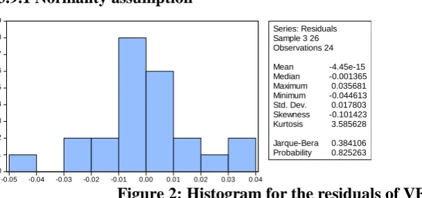
Series: Residuals Sample 3 26 Observations 24 Mean -4.45e-15 Median -0.001365 Maximum 0.035681 Minimum -0.044613 Std. Dev. 0.017803 Skewness -0.101423 Kurtosis 3.585628 Jarque-Bera 0.384106 Probability 0.825263

Figure 2: Histogram for the residuals of VECM model

As it can be seen in figure 2, residuals of the Vector Error Correction model are normally

distributed at 0.05 level of significance.

3.9.2 Serial Correlation

Table12: Breusch-Godfrey Serial Correlation LM Test

Breusch-Godfrey Serial Correlation LM Test:

F-statistic 0.000667 Prob. F(1,14) 0.9798 Obs*R-squared 0.001143 Prob. Chi-Square(1) 0.9730

According to table 12 p value of the LM test is greater than 0.05, which indicates that there is

no serial correlation among the residuals of the VECM model.

3.9.3 Heteroscedasticity

Table 13: ARCH test to check Heteroscedasticity of the residuals

Heteroskedasticity Test: ARCH

F-statistic 0.359142 Prob. F(1,21) 0.5554 Obs*R-squared 0.386732 Prob. Chi-Square(1) 0.5340

As it can be seen in table 13 p value of the ARCH test is greater than 0.05, which indicates

that there is no heteroscedasticity among the residuals of the VECM model.

3.9.4 Stationary Condition

Table 14: Unit Root test Null Hypothesis: RESIDUALS has a unit root

Exogenous: Constant

Lag Length: 2 (Automatic - based on SIC, maxlag=5)

t-Statistic Prob.*

Augmented Dickey-Fuller test statistic -6.685488 0.0000 Test critical values: 1% level -3.788030

5% level -3.012363 10% level -2.646119

As the p value of the unit root test is less than 0.05, we can conclude that the residuals are

stationary. Hence a cointegration relationship exists between variables and the long run

model parameters are consistent and highly efficient.

4. Conclusions

FDI has a huge impact on oil demand in the long run. It has a unitary elastic effect in the

long run and FDI has a small effect in increasing the overall demand for oil in the short run,

with one percent rise in FDI there is only 0.06 increment in demand. FDI is a long term

strategic investment by multinational companies and it may take many years to have an influence in the country’s oil demand. Hence it is unsurprising to have a small effect in the

short run.

Crude oil price has a huge effect in reducing oil demand in the long run, with one percent

increase in oil price there is 3.9 percent reduction in overall demand. In the short run oil

demand will increase by 0.2 percent when price increase by one percent. It seems to be that

when the oil price remain increased for a long period people and the industry may find

alternatives to cut down the expenses by buying less amount of oil.

In the short run one percent rise in population is estimated to have 19 percent increment in oil

demand and in the long run there is a reduction, with one percent rise in population there is 7

percent reduction in overall oil demand. Although population is a significant factor in the

short run, there may be other factors which have more effect on oil demand. For example,

even though the population increases, if the price of the oil is high the demand will reduce in

the long run.

In both long run and short run models for one percent increment in GDP, it is estimated to

have a 1.11 percent and 0.32 percent reduction in the oil demand respectively. Sri Lanka’s

GDP mainly depends on tourism, tea export, apparel, textile, rice production and

other agricultural products. These industries mainly depending on electricity and over the

years proportion of electricity production by coal and hydo has increased while the

proportion of electricity produced by oil has reduced significantly. Hence the industrialization

in Sri Lanka which has increased the GDP has reduced the oil demand in both short run and

long run.

According to variance decomposition, oil demand (LNCON) is relatively less exogenous in

relation to the shocks of macroeconomic variables in the short run because if considering

only two years, the oil demand or the consumption of oil (LNCON) is the most important

Direct Investment (FDI), Gross Domestic Product (GDP), population and oil to the forecast

error variance is 14.26%, 9.68%, 1.82% and 10.23% respectively.

At the end of the period, only 14.96% of variance of consumption is explained by its own

shock. Foreign Direct Investment (FDI), Gross Domestic Product (GDP) and population are

the next most important variables to be considered in explaining the forecast error variance,

which accounts 37.39%, 22.23% and 18.48% impact on consumption of oil respectively. This

implies that Foreign Direct Investment (FDI), Gross Domestic Product (GDP) and population

prove to be the most significant factors that explain the movement in oil demand in the lo ng

run.

References

1. Chan, H. and Lee, S. (1996), “Forecasting the demand for energy in China”, Energy

Journal, Vol. 17 No. 1, pp 19-30.

2. Crompton, Paul & Wu, Yanrui. (2005). Energy Consumption in China: Past Trends

and Future Directions. Energy Economics. 27. 195-208. 10.1016/j.eneco.2004.10.006.

3. Crude oil (petroleum) Monthly Price Sri Lanka Rupee per Barrel, Retrieved from

http://www.indexmundi.com/commodities/?commodity=crudeoil&months=240&curr

ency=lkr

4. Diebold F. X and Kilian L. (2008) “Unit root tests are useful for selecting forecasting models”- Journal of Business and Economic Statistics, 18, 265-273.

5. Dilip Kumar, S. Maheswaran, (2013) "Correlation transmission between crude oil

and Indian markets", South Asian Journal of Global Business Research, Vol. 2

Issue: 2, pp.211-229, https://doi.org/10.1108/SAJGBR-08-2012-0104

6. Engle R.F and Granger C. (1987), “Co-integration and Error Correction Representation, Estimation and Testing”, -Econometrica

7. FDI in Sri Lanka, Retrieved from

http://data.worldbank.org/indicator/BX.KLT.DINV.CD.WD?locations=LK

8. GDP in Sri Lanka, Retrieved from

http://data.worldbank.org/indicator/NY.GDP.MKTP.CD?locations=LK

9. Granger C.W.J. (1969), “Investigating causal Relations by econometric

Models”,-Econometrica

10.Gujarati Damodar N. (2007). United States Military Academy, West Point “Basic Econometrics”- Fourth Edition.

12.Jens Hölscher, Ray Bachan, Andrew Stimpson, (2008) "Oil demand in China: an

econometric approach", International Journal of Emerging Markets, Vol. 3 Issue: 1,

pp.54-70, https://doi.org/10.1108/17468800810849222

13.Kebin He, Hong Huo, Qiang Zhang, Dongquan He, Feng An, Michael Wang, Michael

P. Walsh, Oil consumption and CO2 emissions in China's road transport: current

status, future trends, and policy implications, Energy Policy, Volume 33, Issue 12,

2005, Pages 1499-1507, ISSN 0301-4215,

https://doi.org/10.1016/j.enpol.2004.01.007.

14.Perman, Ma, McGilvray, J. and Common, M. (1999), “Natural Resource and Environmental Economics”,

http://econdse.org/wp-content/uploads/2014/01/perman_et_al_chapters_6_and_7.pdf

15.Samaratunga, R.H.S., (2014). Sri Lanka’s petroleum industry: policy, organization

and challenges . Sri Lanka Journal of Development Administration . 4 , pp . 39–53 .