Violation of Object Functional Unimodality and Evolutionary Algorithms for Optimal Control Problem Solution

2018 IX International Conference on Optimization and Applications (OPTIMA 2018) ISBN: 978-1-60595-587-2

Violation of Object Functional Unimodality and Evolutionary Algorithms

for Optimal Control Problem Solution

Askhat DIVEEV

, Elena SOFRONOVA

_{, and Anton DOTSENKO}

Federal Research Center “Computer Science and Control” of Russian Academy of Sciences, Moscow, Russia

RUDN University, Moscow, Russia Corresponding author

Keywords: Optimal control, Unimodality of functional, Evolutionary algorithms, Phase constraints,

Robotics.

Abstract. _{Some common properties of violation of object function unimodality in optimal con-} trol problems are considered. Phase constraints and control object models for special symmetric systems are considered. It is shown that for a control problem of a group of objects, given in the form of a symmetric system of equations, for certain initial and terminal conditions the functional is not unimodal. It is claimed that for optimal control problems with non-unimodal functionals it is efficient to use evolutionary algorithms. An example of an optimal control problem for a group of symmetric objects with phase constraints resolved by evolutionary and gradient algorithms is provided.

Introduction and Related Work

The most common method to solve the optimal control problem is the transition from the optimal control problem to the nonlinear programming problem and its resolution by classical or modern numerical methods [1]. Previous researches showed that the transition from the optimal control problem to nonlinear programming problem is not difficult, but as the result, we obtain the problem of nonlinear programming of high dimension, and more importantly, in most cases with a non-unimodal objective function. A high dimension of optimization task with a non-unimodal target function does not allow to apply precise methods of global optimization for its resolution [1, 2].

For example, to use a method of non-uniform coverages [3, 4] it is necessary to calculate the estimates of the objective function for each of the areas into which the search space is divided. The number of areas for functional assessment exceeds 2r, where r _{is the dimension of the search space.}

Note, that in case of transformation from the optimal control problem to the nonlinear program- ming problem a situation when r ≥ _{100, is typical. If an object includes} m _{controls and we split the}

control time into k _{intervals then we obtain} r = mk , and the more the k the more accurate the solution is. This problem could be eas- ily solved by modern methods such as stochastic gradient search, which is successfully applied today for the training of artificial neural networks (ANNs), but in this case, we have to make sure that target function is unimodal. Unfortunately, the majority of applied optimal control prob- lems have non-unimodal functionals, such as problems with phase constraints, which one often

1

2 *

encounters in robotics [5]-[6].

This circumstance causes a high popularity of evolutionary algorithms (EAs) in recent years that can be attributed to the methods of adaptive random search. These methods are not sensitive to the dimension of the problem and the form of the functional. But it is worth noting that it is almost always difficult to measure how far a solution lies from the optimal one.

In this paper, we consider some conditions under which the functional in the optimal control problem loses the property of unimodality. We introduce a time-independent measure in the space of solutions of differential equations and prove a theorem that under certain conditions, the presence of phase constraints leads to non-unimodality of the functional. We further consider the control problem for a group of objects and show that with a time-dependent measure, each object is a phase constraint for other objects, and for special symmetric systems under certain initial and terminal conditions the functional is always non-unimodal.

Theoretic Results

Solution of the System of Differential Equations in Optimal Control Problem

Consider a system of n ordinary differential equations in Cauchy form with free control vector

u in the right part

˙

x=f(x,u), (1)

where x∈_Rn_,u∈

Rm.Let the values of a control vector be defined as time functions

u=v(t), (2)

where u= [u1. . . um]T,v= [v1(t). . . vm(t)]T. Consider a set of these functions

V ={vi(t) :i= 1, . . . , M}, (3)

with the solution x(t) of the system of differential equations (1),

˙

x=f(x,vi(t)),vi(t)∈V, (4)

if it starts at the moment t0 = 0 from the point

x0 = [x0₁. . . x0_n]T, (5)

and finish at the moment ti at the point

xf = [xf₁. . . xf_n]T,xf 6=x0. (6)

Let the following condition be satisfied

ti ≤t+, i= 1, . . . , M. (7)

We add the terminal stability conditions to all of the solutions of the system

e

xi(t) = (

xi_{(t), t < t} i

xf_,otherwise , (8)

where xi_{(t) is a solution of the system (1) with control u=v}i_(t). Let

e

X ={xi(t) :i= 1, . . . , M} (9)

be a set of solutions of the system (1) with additional terminal stability conditions (8). Then we introduce the distance between two solutions from Xe

∆(xi_,xj_{) = max{max}

α∈[0;t+_]min_β∈[0;t+_]k

e

xi_(α)−

e

xj_(β)k,

max_α∈[0;t+_]min_β∈[0;t+_]k

e

xi_(β)−

e

xj_(α)k,}

(10)

where kxk is any convex norm of vector in _Rn_{, e.g.,}

kxk∞= max{|xi|:i= 1, . . . , n} or kxk2 = v u u t

n

X

i=1 x2

i.

Definition 1. Fundamental sequenceF(xi_,xj_{) of solutions is a set of solutions{}

e

xik _{:k= 0, . . . , L+}

1,_exi0 ₌

e

xi_,

e

xiL+1 ₌

e

xj_{} ⊆}

e

X,for which following conditions are met:

∆(xik_,xik+1_{)< ε, k= 0, . . . , L, (11)}

where ε is a small value.

Definition 2. The solution set X is continuous, if for any two solutions from the set _exi,x_ej ⊆ Xe and some small positive value we can get a fundamental sequence F(xi_,xj_)⊆

e X.

Definition 3. ε-neighborhood of solutions in continuous solution set is a set of all solutions, with the following conditions fulfilled

∆(_ex,x_ej)≤ε.

Let the nonnegative functional be given on the continuous solution set

J(_ex(t)) :_Rn →_R1_{. (12)}

Let the functional have the following property: for any solution_exi _∈

e

X and given positive value δ there exist a solutionx_ej _∈

e

X and the value ε >0 such that the following conditions are satisfied

|J(x_ei(t))−J(_exj(t))|< δ,∆(x_ei,_exj)< ε. (13)

It means that the functional has continuous values of estimates on the set of solutions X.e

Theorem 1. If on a continuous set of solutions X a functional has a unimodal minimum for ae solutionx_e−∈X, then for any solutione x_ei ∈X,e x_ei 6=_ex− we can always get a fundamental sequence

{_exik _{:k = 0, . . . , L+ 1,}

e

xi0 ₌

e

x−,_exiL+1 ₌

e

xi} ⊆Xe (14)

under the following conditions

J(x_eik_(t))≤J(

e

xik+1_(t)).

Proof. Consider a solution _exi _∈

e

X. In its ε-neighborhood we find a solution _exi1 _{with minimal}

estimation of functional J(_exi1_{(t)) ≤ J(}

e

xi_{(t)). If such solution does not exist, then the solution}

e

xi ∈ X is a local minimum. According to the conditions the solution does not coincide with ae minimum _ex− ∈ X which means that the functional is not unimodal. Therefore, that solutione exists. Now consider ε - neighborhood of a solution_exi1 _{and we find in its neighborhood a solution}

e

xi2_{, for which the functional has a smaller value, J(}

e

xi2_{(t))≤ J(}

e

xi1_{(t)). Repeat this process until}

we find the minimum of the functional _ex− ∈ X in this neighborhood. All solutions found ine ε -neighborhood taken in the reverse order will be the fundamental sequence (14). The theorem is proved.

Theorem 2. Let in continuous solution set X exist two solutionse x_ei,_exj ∈X such that for any fun-e damental sequence F(_exi_,

e

xj_)⊆

e

X there always exist a solution _exk_∈F(

e

xi_,

e

xj_{) under the following} conditions

J(x_ek(t))> J(x_ei(t)) and J(_exk(t))> J(_exj(t)). (15)

Then the functional is not unimodal for the minimum problem

J(_ex(t))→min e X

.

Proof. Consider ε-neighborhood of each solution _exi,_exj ∈X. We find solutions in these neighbor-e hoods with smaller values of functional estimates J(_exi1_(t)) ≤ _J(

e

xi_{(t)) and J(}

e

xj1_(t)) ≤ _J(

e

xj_(t)). Now consider ε-neighborhoods of the found solutions _exi1_,

e

xj1 _∈

e

X. We find again solutions with smaller values of functional estimates in their ε-neighborhoods. Repeat this process until we find solutions _exiL _and

e

xiK _{with ε-neighborhoods where no solutions exist with smaller values of}

func-tional estimates. If these minimums coincide,_exiL₌

e

xiK _{, than it means that for solutions}

e

xi,_exj ∈Xe we can build a fundamental sequence for which the conditions(15) of the theorem are not satisfied. Hence these solutions don’t coincide _exiL 6₌

e

xjK_{. It means that functional for a solution set is not}

unimodal. The theorem is proved.

Consider projections of solutions in _R2_{. We consider only two components from all of the} components of solutions _ex = [x_e1. . .xen]

T_{. Let it be components}

e

x1,xe2. So we consider subspace

R2 inRn with a transformation

y=Cx, (16)

where x∈_Rn_,y∈ R2,

C=

1 0 0. . .0 0 1 0. . .0

.

Let the closed area be defined in D⊆_R2_{. We determine a size of the area from its diameter.}

Definition 4. The constructive diameter of a closed area is called the diameter of the maximum sphere inscribed in this area.

Let S be a sphere of maximal size included in D

S(x1, x2) = (x1−x∗1) 2

+ (x2−x∗2) 2₋

R2 = 0,

where x∗₁, x∗₂ are the coordinates of the center of the circle. Then the diameter of the area D is equal 2R and ∀x1, x2, with S(x1, x2)≤0, x1, x2 ∈D.

Consider a set of solutions in _R2 from the point y0 =Cx0 to the point yf =Cxf. A solution set in _R2 _{starting from y}0 _{and finishing iny}f_{, and complemented by terminal stability conditions} (8) we denote as Y.e

Theorem 3. If in a solution set Y exist two solutionse _eyi and _eyj with the distance ∆(y_ei,_eyj), then it is impossible to place the area with the diameter 2R >∆(_eyi,_eyj) between these solutions in such way that the solutions y_ei _and

e

yj _{did not cross this area.}

Let’s set an area D ⊆_R2 _{with diameter 2R. Let’s take a point (x}p 1, x

p

1)∈ D and build a polar coordinate system {ρ, ϕ} with the center at a point (xp₁, xp₁). For transformation from Cartesian coordinates in _R2 to polar coordinates we use the following equations

ρ=p(x1−xp1)2+ (x2 −xp2)2, (17)

ϕ(x) =       

arctan(x2−xp2

x1−xp1

)±2π, if x1−xp1 >0

sgn(x2−xp2)π−arctan( x2−xp2

x1−xp1)±2π, if x1−x

p 1 <0.

sgn(x2−xp2) π

2 ±2π, if x1−x

p 1 = 0

(18)

We transform all solutionsy_ek_{(t) = [}

e xk

1(t)xe

k

2(t)]T fromY to polar coordinatese {ρ, ϕ}and obtain solutions in the form _epk_{(t) = [}

e ρk_(t)

e ϕk_(t)]T_.

Theorem 4. Let in a solution setY starting at the moment 0 in the pointe y0 = [x0₁x0₂]T and ending at the momenttf passing the pointyf = [xf1x

f

2]T, has two solutions ey

i_,

e

yj, which do not cross the area D with construct diameter 2R, or ∀t ∈ [0, tf] S(xi1(t), xi2(t)) > 0 and S(x

j 1(t), x

j

2(t)) > 0, where S(x1, x2) = (x1−x∗1)2+ (x2−x∗2)2−R2 = 0,, x∗1, x∗2 ∈D for which the following conditions are met

|ϕ_ei(tf)−ϕe

j_(t

f)|= 2π, (19)

where ϕ_ei(t),ϕ_ej(t) are angular components in the representation of solutions y_ei,y_ej in polar coor-dinates p_ei_{(t) = [}

e ρi_(t)

e ϕi_(t)]T_,

e

pj_{(t) = [}

e ρj_(t)

e

ϕj_(t)]T _{by equations (17), (18). These is enough that} distance between solutions _eyi_,

e

yj _{was not less than 2R}

∆(y_ei,y_ej)≥2R.

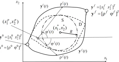
Proof. Consider the Fig. 1

Fig.1 shows the case, where angles ϕ_ei_(t

f) andϕe

j_(t

f) differ in value 2π. The solutions in polar coordinates _epi_{(t) = [}

e ρi_(t)

e ϕi_(t)]T

e

pj_{(t) = [}

e ρj_(t)

e

ϕi_(t)]T _{start at the momentt = 0 with an angle ϕ}0 and finish with an angle ϕf, here a solution p_ei(t) moves in clockwise order, and a solution p_ej(t) moves contra clockwise. Because ϕ0 _{> ϕ}f_{, and the solution}

e

pj_{(t) moves toward increasing of an} angle, then ϕ_ej_{(0) =ϕ}0_{−2π. Hence,}

e

ϕj(tf) =ϕ0+ (ϕf −ϕ0+ 2π)

.

e

Figure 1. Solutions in polar coordinates.

From these equations we obtain |ϕ_ei_(t

f)−ϕe

j_(t

f)| = 2π. According to the theorem 3 if the distance between solutions is less than 2R, than these solutions will cross the area D and will not meet the conditions of the theorem. The theorem is proved.

Let us introduce a functional (12) on the set of solutions. Assume an area D ⊆ _R2 _defined in _R2 _{such that if a solution}

e

yk_{(t) crosses the area D, then the value of the functional increases} significantly: ∀_ey(t)∈Y a following condition fulfilled J(_ey(t))< J(_eyk(t)), if∀t ∈[0;tf] ∀ye(t)∈/ D and ∃t0 ∈[0;tf] such that∀ey

k_(t0_)∈D.

Let us assume that in a solution set Y there exist two solutionse e

yi_{(t) and}

e

yj_{(t), which do} not cross the area D and fulfill (16). It means that any fundamental sequence between these solutions will contain a solution _eyk_{(t) which crosses the area}

e

D, therefore J(_eyk_{(t))< J(}

e

yi_{(t)) and}

J(y_ek_{(t))> J(}

e

yj_{(t)). According to the theorem 2 the functional will not be unimodal on a set of} solutionsY.e

Symmetrical Systems

Definition 5.If the system of differential equations ˙x = f(x,u_e(t)) has a partial solution x_e(t), with fulfilled boundary conditions: _ex(0) = x0, _ex(tf) = xf, and the partial solution of the system of differential equations x˙ =f(x,−u_e(tf −t)) with initial conditions xe(0) = x

f _is

e

x(tf −t), then such system of differential conditions is called symmetrical system.

Assertion 1. A system of differential equations ˙x=_eu(t) is symmetrical.

Proof. After integration of the system, we get

e

x(t) = _ev(t) +c.

At t= 0, c=x0 ₋ e

v(0), therefore the partial solution of the system is

e

x(t) = _ev(t) +x0−v_e(0).

From the solution, we obtain at the moment t=tf

xf =_ev(tf) +x0−ve(0).

Now we consider an equation

˙

To solve the equation denote z =tf −t, that why

−

Z

e

u(tf −t)dt=

Z

e

u(z)dz

or

e e

x(z) = _ev(z) +c,

e e

x(t) = _ev(tf −t) +c.

By definition at t = 0 e e

x(0) =xf_{, therefore we obtain}

c=e e

x(0)−_ev(tf) = xf −xf +x0−ev(0) = x 0₋

e

v(0)

and

e e

x(t) =v_e(tf −t) +x0−ev(0)

or

e e

x(t) =x_e(tf −t).

Q.E.D.

From the statement 1 follows that the system of differential equations

˙

x=B(x)_eu(t)

where B(x) is a functionality matrix with dimension n×m which is symmetric.

Lemma 1.

Z tf

0

f0(ex(t))dt = Z tf

0

f0(ex(tf −t))dt.

Proof.

Z tf

0

f0(xe(tf −t))dt =− Z zf

z0

f0(ex(z))dz

where z =tf −t, dz =−dt, z0 =tf, zf = 0. Therefore

−

Z zf

z0

f0(ex(z))dz =− Z 0

tf

f0(ex(z))dz =− Z tf

0

f0(ex(z))dz.

Q.E.D.

Really _ex(tf − t)) is the same trajectory as xe(t)) in R

n _{but with movement in the opposite}

direction.

Theorem 5. If _eu(t) is a solution of the optimal control problem

˙

x=f(x, u),

x(0) =x0,x(tf) =xf, (20)

Z tf

0

f0(x)dt→min,

where ˙x=f(x, u) is a symmetric system of differential equations. Then −u_e(tf −t)) is a solution of the optimal control problem

˙

x=f(x, u),

x(0) =xf,x(tf) =x0, (21)

Z tf

0

f0(x)dt→min.

Proof. From the statement 1 it follows that if x_e(t) is a solution of the system with boundary conditions (20), than _ex(tf −t) is a solution of system with boundary conditions (21) and vice versa. Since the lemma 1 it follows that values of functional for both problems is equal. If there were a controle

e

u(t) for the boundary condition problem (21) which would provide the solution e e

x(t) with smaller value of a functional, then there would also exist a solution e

e

x(tf −t) with smaller value of a functional for the problem with boundary conditions (20). In this case u_e(t) is not a solution for the optimal control problem. Hence, there is no such solution, which means that

−e e

u(tf −t) is the solution of the optimal control problem with boundary conditions (21). Q.E.D.

The theorem 5 shows why these systems are called symmetrical. For these systems, the optimal trajectory from the a A to a point B coincides with the optimal trajectory from the point B to the point A.

Theorem 6. In the problem of optimal control of two objects

˙

xi =f(xi,ui),

xi(0) =x0,i,xi(tf) =xf,i, (22)

ui ∈U⊆_Rm,

where i= 1,2,

Z tf

0

f0(x1,x2)dt →min,

with boundary conditions

xf,1 =x0,2 and xf,2 =x0,1 (23)

and symmetric identical models of objects (22) there are at least two optimal controls that are solutions of the problem.

Proof. Let _eu(t) be a solution of the optimal control problem. Then, according to theorem 4,

−e e

u(tf −t) it is also the optimal control for the problem with boundary conditionsx0,1 =xf,1 and

x0,2 _=xf,2_.

Since (23) we obtain

x0,1 =xf,1 =x0,2,x0,2 =xf,2 =x0,1.

Since the objects are the same, we get the same optimal control problem. Therefore−u_e(tf−t) is also a solution to the same optimal control problem. Q.E.D.

One can add to the problem conditions of absence of rapprochement among objects.

R2 −

v u u t

k

X

i=1 (y1

i(t)−yi2(t))≤0,∀t∈[0;tf],

where yi_{(t) =Cx}i_{(t), i= 1,2,C is a (k×n) matrix.}

Computational Experiment

Let us consider the problem of optimal control of a group of N objects with phase constraints. Given a mathematical model of a mobile robot

˙

x1+(j−1)n= 0.5(u1+(j−1)m+u2+(j−1)m) cos(x3+(j−1)n) ˙

x2+(j−1)n= 0.5(u1+(j−1)m+u2+(j−1)m) sin(x3+(j−1)n) ˙

x3+(j−1)n= 0.5(u1+(j−1)m−u2+(j−1)m)

(24)

where n is a dimension of model for one robot, in our case, n = 3, m is a dimension of control vector of one robot, here m = 2, x= [x1, . . . , x3+(N−1)n]T, is a vector of state space of the group of robots, u = [u1, . . . , u2+(N−1)m]T is a vector of control of the group of robots,j = 1, . . . , N, N is a number of robots in the group.

For the group of four robots,N = 4, we have 12 equations in the system (24) or 12 components of the state space and 8 components of the control vector

The controls values are limited

u−_i ≤ui+(j−1)m ≤u+i , i= 1, . . . , m, j= 1, . . . , N. (25)

Initial states of robots are given

xi+(j−1)n(0) =x0i+(j−1)n, i= 1, . . . , n, j = 1, . . . , N. (26)

There is a static phase constraint

β(x) = r2−(x∗₁−x1+(j−1)n)2−(x∗2−x2+(j1)n)

2 _{≤0, j = 1, . . . , N, (27)}

where r is some given positive value, x∗₁, x∗₂ are the coordinates of static phase constraint center. To avoid collisions between the robots, we provide the following dynamic phase constraints

δk(x(t)) =r20−(x1+(j−1)n−x1+(i−1)n)2−(x2+(j−1)n−x1+(i−1)n)2 ≤0, (28)

where

k=i−j+ (j−1)(N −0.5j), (29)

r0 is a given positive value, j = 1, . . . , N −1, i=j+ 1, . . . , N.

From (29) we obtain the maximum number of checks of dynamic phase restrictions atj =N−1 and i=N:

k =N −N + 1 + (N −1−1)(N −0.5(N −1)) = 1 + (N−2)(0.5N + 0.5) =

= 1 + 0.5(N2−N −2) = 0.5(N2−N) = 0.5N(N −1).

As result, we obtain the number of combinations from N on 2. Terminal states of robots are

xi+(j−1)n=x f

i+(j−1)n, i= 1, . . . , n, j = 1, . . . , N. (30)

Quality criterion is

e

J =tf →min, (31)

where tf time of the end of simulation process

tf =

(

t,if t < t+ _{and max}

||∆x(i+j−1)n(t)||2 :j = 1, . . . , N < ε

t+_,otherwise (32)

||∆x(i+j−1)n(t)||2 = v u u t

n

X

i=1

(x_i+(j−1)n(t)−xf_i+(j−1)n)2_,

t+ _{is a maximum possible control time, ε is a small positive value.}

We provide phase constraints in quality criterion using Heaviside function

J =tf + N

X

j=1 Z tf

0

ϑ(β(x(t)))dt+ N−1 X

i=1 N

X

j=i+1 Z tf

0

ϑ(δk(x(t)))dt→min, (33)

where β(x(t)) and δk(x(t) are determined by formulas (27) and (28) respectively,

ϑ(A) = (

1,if A_>1 0,otherwise.

We used the following constant values of parameters of the model: n = 3,

m = 2, N = 4, x0₁ = 0, x0₂ = 0, x0₃ = 0, x₄0 = 0, x0₅ = 10, x0₆ = 0, x0₇ = 10, x0₈ = 0,

x0₉ = 0, x0₁0 = 10, x0₁1 = 10, x0₁2 = 0, xf₁ = 10, xf₂ = 10, x0₃ = 0, x104 = 10, x05 = 0,

x0₆ = 0, x0₇ = 0, x0₈ = 10, x0₉ = 0, x0₁0 = 0, x0₁1 = 0, x0₁2 = 0, t+ = 2.8, ε= 0.01, u−₁ =−10, u−₂ =−10, u+₁ = 10, u+₂ =−10.

To solve the optimal control problem(24)-(33) of infinite dimension we transform it to nonlinear programming problem of finite dimension. We select interval ∆t and split the time of control onto L intervals

L= jt+

∆t k

+ 1.

On each interval, we approximate control of the object by functions depending on finite number parameters.

We set obtained control to zero by approximation functions if it satisfies the following restric-tions

ui(t) =

  

 

u+_,if e

ui(t)≥u+

u−,if _eui(t)≤u−, i= 1, . . . , mN,

e

ui(t),otherwise

(34)

where _eui(t) is an approximating function.

For approximation of control, we use the fourth order Hermit polynomial, Bezier curve func-tions, cubic polynomials, piecewise linear function, and piecewise constant function.

We solved the nonlinear programming problem by five well known algorithms: algorithm of fast gradient descent (FGDA) [7, 8], particle swarm optimization (PSO) [9, 10], genetic algorithm (GA) [11, 12], random search (RS) and adaptive algorithm of stochastic gradient (ADAM) [13]. The quality of search of evolutionary algorithms depends on the quantity of possible solutions in the initial set and the number of evolutionary transformations, therefore we estimate the effectiveness of algorithms by the number of calculations of target function and by the best-found solution. Note, that for the calculation of one value of a gradient the number of calculations of target function is equal to the dimension of search space. The results of computations are presented in Table 1.

In the Table 1 column one shows the methods of transformation to the nonlinear programming problem: Cube is a cubic polynomial, Hermit is a Hermit polynomial, Bezier is a Bezier polynomial, Linear is an approximation by linear functions. Constant is an approximation by piecewise constant functions. Note, that values marked with * are given in series of 10 experiments. As it can be seen from Table 1, evolutionary algorithms perform much better than other algorithms. The best-found solution has the value of functional 3.4987. It was obtained by PSO algorithm.

The best found solution is

e

q= [−19.386−15.424−19.758−11.291−19.995−7.217 15.213 19.166 14.471−17.018−0.104 19.665 5.433−19.988−11.661−16.911

19.884 19.914 3.138−11.472−19.991−11.169 13.684−7.503

−14.478−11.982−17.202 16.257 19.916 19.959 19.839−19.877 4.265−18.173−10.405−19.970−19.448 8.587 12.291 18.394

14.360 9.441 19.842−19.933−18.911−8.419 4.644 8.434 11.161 12.217 15.492−7.754−18.977−10.800−10.910 18.196

−18.076−19.996 13.777−1.032 16.507 11.284 9.916−19.273

−14.311−19.925−9.799−19.950−0.301−17.725 19.832 12.084

−20.000−10.225 18.007 11.890 19.008 −17.670−19.971−7.332

−19.675−19.948 18.937 10.148 16.420 14.907 19.959 3.142].T

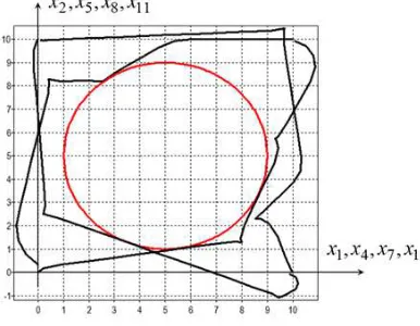
Fig. 2 shows obtained trajectories of four mobile robots on the plane. In the state vector for all robots these are coordinates (x1, x2), (x4, x5), (x7, x8), (x10, x11). All control objects have reached terminal points and have not broken static constraints. The forms of obtained trajectories are evidently not optimal and can be improved.

Conclusion

The study considers conditions under which functionals in optimal control problems with phase constraints and control of a group of objects are not unimodal. As an example, an optimal control problem with phase constraints for 4 mobile robots is solved. Gradient methods in such problems showed unstable results. The values of functional in different series of experiments differ in more

Table 1. Results of experiment.

Method of transformation

Best value of functional*

Average mean*

Root mean square deviation*

Quantity of calculations of

functional PSO

Cube 7.6864 8.917237 0.892737 2500511

Hermit 5.1408 9.686063 2.117146 2500511

Bezier 4.1660 8.023544 2.758620 2500511

Linear 3.4987 5.497326 1.427645 2500511

Constant 3.8021 5.437543 1.165168 2500511

RS

Cube 12.0909 13.080324 0.868641 2500511

Hermit 14.0148 15.897309 1.245307 2500511

Bezier 9.2596 14.768950 2.760597 2500511

Linear 5.6273 12.238500 4.751106 2500511

Constant 9.4286 12.790501 2.640101 2500511

GA

Cube 12.0909 13.080324 0.868641 2500511

Hermit 14.0148 15.897309 1.245307 2500511

Bezier 9.2596 14.768950 2.760597 2500511

Linear 5.6273 12.238500 4.751106 2500511

Constant 9.4286 12.790501 2.640101 2500511

FGDA

Cube 18.5099 21.604358 3.912750 2594575

Hermit 18.4947 21.301057 1.686402 2591268

Bezier 22.3052 23.314141 1.006914 2606501

Linear 21.4992 22.366198 0.942382 2743742

Constant 23.5008 24.782348 0.779497 2715137

ADAM

Cube 18.0045 18.743846 0.905551 2550251

Hermit 13.8628 16.149400 2.229859 2550261

Bezier 6.0134 8.905433 1.194444 2550261

Linear 7.6490 9.294152 1.144378 2522661

Constant 7.4528 8.841364 1.026492 2522661

Figure 2. Trajectories of the best obtained solution.

than two times. It is experimentally shown that evolutionary algorithms are more suitable for the solution of optimal control problems.

Acknowledgements

This work was supported by Russian Foundation for Basic Research, Projects 16–29–04224– ofim, 17–08–01203–a, 18–29–03061–mk.

References

[1] W. Esposito and C. Floudas Deterministic Global Optimization in Nonlinear Optimal Control Problems. J. Glob. Optim. 17 (2000) 97-126.

[2] M. Gaviano and D. Lera A global minimization algorithm for Lipschitz functions. Optimization Letters. 2. (2008) 1-13.

[3] Y. Evtushenko and M. Posypkin A deterministic algorithm for global multi-objective opti-mization. J. Optimization Methods and Software. 29. (2014) 1005-1019.

[4] Y. Evtushenko and M. Posypkin Method of Non-uniform Coverages to Solve the Multicriteria Optimization Problems with Guaranteed Accuracy. Automation and Remote Control. 75. (2014) 1025-1040.

[5] A. Arutyunov and D. Karamzin Non-degenerate Necessary Optimality Conditions for the Op-timal Control Problem with Equality-type State Constraints. Journal of Global Optimization. 64. (2016) 623-647.

[6] A. Diveev, E. Shmalko, and D. Zakharov Acceleration of the multilayer network operator method using MPI for mobile robot team control synthesis. Procedia Computer Science. (2017) 158-163.

[7] A. Patrascu and I. Necoara Efficient random coordinate descent algorithms for large-scale structured nonconvex optimization. J. Glob. Optim. 61. (2015) 19-46.

[8] S. Puechmorel and D. Delahaye Order statistics and region-based evolutionary computation. J. Glob. Optim. 59. (2014) 107-130.

[9] H. W. Y. Jie, J. Zhao, and J. L. Ding An efficient multi-objective PSO algorithm assisted by Kriging metamodel for expensive black-box problems. J. Glob. Optim. 67. (2017) 399-423. [10] J. Kennedy and R. Eberhart Particle Swarm Optimization. In: Proceedings of IEEE

Interna-tional Conference on Neural Networks IV. (1995) 1942-1948.

[11] D. Fogel Asymptotic convergence properties of genetic algorithms. Cybernetics and Systems. 25. (1994) 389-407.

[12] G. Rudolph Convergence Analysis of Canonical Genetic Algorithms. IEEE Transactions on Neural Networks. (1994) 96-101.

[13] D. Kingma and J. Ba ADAM: A Method for Stochastic Optimization. In: 3rd International Conference for Learning Representations, San Diego (2015) 15.