A robust test for mean change in dependent observations

(1)

R E S E A R C H

Open Access

A robust test for mean change in dependent

observations

Ruibing Qin

1*

_{and Weiqi Liu}

2

*_{Correspondence:} [email protected]

1_{School of Mathematical Science,} Shanxi University, Taiyuan, Shanxi 030006, P.R. China

Full list of author information is available at the end of the article

Abstract

A robust test based on the indicators of the data minus the sample median is proposed to detect the change in the mean of

α

-mixing stochastic sequences. The asymptotic distribution of the test is established under the null hypothesis that the mean

μ

remains as a constant. The consistency of the proposed test is also obtained under the alternative hypothesis that

μ

changes at some unknown time. Simulations demonstrate that the test behaves well for heavy-tailed sequences.

MSC: Primary 62G08; 62M10

Keywords: change point; median; robust test; consistency

1 Introduction

The problem of a mean change at an unknown location in a sequence of observations has received considerable attention in the literature. For example, Sen and Srivastava [], Hawkins [], Worsley [] proposed tests for a change in the mean of normal series. Yao [] proposed some estimators of the change point in a sequence of independent variables. For serially correlated data, Bai [] considered the estimation of the change point in linear processes. Horváth and Kokoszka [] gave an estimator of the change point in a long-range dependent series.

Most of the existing results in the statistic and econometric literature have concentrated on the case that the innovations are Gaussian. In fact, many economic and financial time series can be very heavy-tailed with infinite variances; seee.g.Mittnik and Rachev []. Therefore, the series with infinite-variance innovations aroused a great deal of interest of researchers in statistics, such as Phillips [], Horváth and Kokoskza [], Han and Tian [, ]. It is more efficient to construct robust procedures for heavy-tailed innovations, such as theMprocedures in Hušková [, ] and the references therein. De Jonget al.

[] proposed a robust KPSS test based on the ‘sign’ of the data minus the sample median, which behaves rather well for heavy-tailed series. In this paper, we shall construct a robust test for the mean change in a sequence.

The rest of this paper is organized as follows: Section  introduces the models and nec-essary assumptions for the asymptotic properties. Section  gives the asymptotic distri-bution and the consistency of the test proposed in the paper. In Section , we shall show the statistical behaviors through simulations. All mathematical proofs are collected in the Appendix.

(2)

2 Model and assumptions

In the following, we concentrate ourselves on the model as follows:

Yt=μ(t) +Xt, μ(t) =

μ, t≤k,

μ, t>k, ()

wherekis the change point.

In order to obtain the weak convergence and the convergence rate, X(t) satisﬁes the following.

Assumption 

. TheXjare strictly stationary random variables, andμ˜is the unique population median of{Xt, ≤t≤T}.

. TheXjare strong (α-) mixing, and for some ﬁniter> andC> , and for some

η> ,α(m)≤Cm–r/(r–)–η_.

. Xj–μ˜ has a continuous densityf(x)in a neighborhood[–η,η]of  for someη> , andinfx∈[–η,η]f(x) > .

. σ_∈_(,_{∞), where}_σ_{is deﬁned as follows:}

σ= lim T→∞E

T–/

T

t=

sgn(Xt–μ˜)

 .

To derive the CLT of sign-transformed data, we need a kernel estimator, so we make the following assumption on the kernel function.

Assumption 

. k(·)satisﬁes_–∞_∞|ψ(ξ)|dξ<∞, where

ψ(ξ)dξ= (π)–

∞

–∞k(x)

exp(–itξ)dx.

. k(x)is continuous at all but a ﬁnite number of points,k(x) =k(–x),|k(x)| ≤l(x) wherel(x)is nondecreasing and_∞|l(x)|dx≤ ∞, andk() = .

. γT/T→, andγT→ ∞asT→ ∞.

Remark  De Jonget al.[] test the stationarity of a sequence under Assumption . We detect change in the mean of a sequence, so Assumption  holds under the null hypothesis and the alternative one. Since there is no moment condition forXtin Assumption , even Cauchy series are allowed. Theα-mixing sequences can include many time series, such as autoregressive or heteroscedastic series under some conditions. Assumption  allows some choices such as the Bartlett, quadratic spectral, and Parzen kernel functions.

3 Main results

LetmT=med{Y, . . . ,YT}. Then we transform the dataY, . . . ,YT into the indicator data sgn(Yt–mT), wheresgn(x) =  ifx> ,sgn(x) = – ifx< ,sgn(x) =  ifx= . Based on these indicator data, De Jonget al.[] replaceˆt=Yt–YT¯ withsgn(Yt–mT) in the usual

(3)

The popularly used test to detect a mean change is based on the CUSUM type as follows:

T(τ) =

[Tτ][T( –τ)]

T

 [Tτ]

[Tτ]

t=

Yt–

 [T( –τ)]

T

t=[Tτ]+

Yt

. ()

We rewriteT(τ) underHas

T(τ) =

[Tτ][T( –τ)]

T

 [Tτ]

[Tτ]

t=

(Yt–YT¯ ) –  [T( –τ)]

T

t=[Tτ]+

(Yt–YT¯ )

, ()

According to the idea of De Jonget al.[], replaceˆt=Yt–YT¯ withsgn(Yt–mT) in ();

then we get a robust version of CUSUM as follows:

T=

[Tτ][T( –τ)]

T

 [Tτ]

[Tτ]

t=

sgn(Yt–mT) –  [T( –τ)]

T

t=[Tτ]+

sgn(Yt–mT)

. ()

Then the test statistic proposed in this paper is

T=T/σ–max

τ∈(,)

_T(τ) . ()

Under Assumptions , , we can obtain two asymptotic results as follows.

Theorem  If Assumptions, hold,then under the null hypothesis H,we have

T/σ–max

τ∈(,)|T| ⇒ _τ∈sup_(,)

W(τ) –τW() , as T→ ∞, ()

where ‘⇒’ stands for the weak convergence.

Under the alternative hypothesisH, a change in the mean happens at some time, we denote the time as [Tτ]. LetF(·) be the common distribution function ofXt andμ∗be the median of

F∗(·) =τF(·–μ) + ( –τ)F(·–μ). ()

Then we have the following.

Theorem  If Assumptions, hold,then under the alternative hypothesis H,we have

max

τ∈(,)

T(τ) P

→τ( –τ)||, ()

where=F(μ∗–μ) –F(μ∗–μ).

Remark  By Theorem , we rejectHifT>cp, where the critic valuecp is the ( –p)

quantile of the Kolmogorov-Smirnov distribution. By Theorem ,Tis consistent

(4)

In order to apply the test in (), we employ the HAC estimator instead of the unknown

σas

ˆ

σ_T=T– T

i=

T

j=

k(i–j)/γT

sgn(Yi–mT)sgn(Yj–mT), ()

then the following theorem proves two results of the estimatorσˆ_TunderHandHA,

re-spectively.

Theorem  (i)Assuming that the conditions of Theoremhold,then we have,as T→ ∞,

ˆ

σ_T→P σ. ()

(ii)Assuming that the conditions of Theoremhold,then we have,as T→ ∞,

ˆ

σ_T→P σ_, ()

whereσ_is deﬁned as follows:

σ_= lim T→∞E

T–/

T

t=

sgnYt–μ∗ 

.

4 Simulation and empirical application

4.1 Simulation

In this section, we present Monte Carlo simulations to investigate the size and the power of the robust CUSUM and the ordinary CUSUM tests. Since a lot of information has been lost during the inference by using the indicator data instead of the original data, so we are concerned whether the indicator CUSUM test is robust to the heavy-tailed sequences; moreover, we may ask: how large is the loss in power in using indicators when the data has a nearly normal distribution? The HAC estimatorσˆin the robust CUSUM test is a kernel estimator, so it is important to analyze whether the performance is aﬀected by the choice of the kernel functionk(·) and the bandwidthγT.

We consider the model as follows:

Yt=

 +Xt, t≤Tτ,

μ+Xt, t>Tτ,

()

Xt is an autoregressive processXt= .Xt–+et, where the{et} are independent noise

generated by the program from JP Nolan. We vary the tail thickness of{et}by the diﬀerent characteristic indicesα= ., ., ., ., respectively. Accordingly the break times are

τ= ., ., respectively. During the simulations, we adopt . as the asymptotic critical value ofsup_τ∈_(,)|W(τ) –τW()|at % for the various sample sizesT= , , ,. First, we consider the size of the tests. Tables  and  report the results whenσ _are estimated by the Bartlett kernel and the quadratic spectral kernel with the bandwidth

γT= [(T/)/] andγT= [(T/)/], respectively, in , repetitions. From Tables 

(5)

[image:5.595.152.441.106.240.2]

Table 1 The empirical levels of the robust CUSUM test and the CUSUM test for dependent innovations

CUSUM RCUSUM

T = 300 T = 500 T = 1,000 T = 300 T = 500 T = 1,000

The tests based on the Bartlett kernel function

α= 1.97 0.045 0.026 0.036 0.042 0.046 0.059 α= 1.83 0.028 0.028 0.033 0.037 0.032 0.043 α= 1.41 0.010 0.010 0.025 0.030 0.036 0.044 α= 1.14 0.005 0.010 0.008 0.045 0.049 0.048 The tests based on the quadratic spectral kernel function

α= 1.97 0.471 0.491 0.489 0.068 0.048 0.050 α= 1.83 0.428 0.462 0.478 0.062 0.077 0.063 α= 1.41 0.458 0.449 0.486 0.066 0.072 0.053 α= 1.14 0.474 0.476 0.507 0.083 0.073 0.055

The values in Table 1 are based on the bandwidthγT= [4(T/100)1/4].

Table 2 The empirical levels of the robust CUSUM test and the CUSUM test for dependent innovations

T = 300 T = 500 T = 1,000 T = 300 T = 500 T = 1,000

The tests based on the Bartlett kernel function

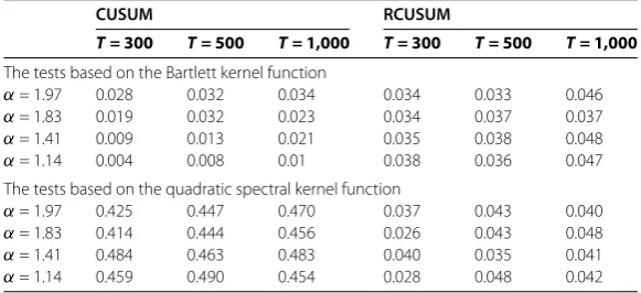
α= 1.97 0.028 0.032 0.034 0.034 0.033 0.046 α= 1.83 0.019 0.032 0.023 0.034 0.037 0.037 α= 1.41 0.009 0.013 0.021 0.035 0.038 0.048 α= 1.14 0.004 0.008 0.01 0.038 0.036 0.047 The tests based on the quadratic spectral kernel function

α= 1.97 0.425 0.447 0.470 0.037 0.043 0.040 α= 1.83 0.414 0.444 0.456 0.026 0.043 0.048 α= 1.41 0.484 0.463 0.483 0.040 0.035 0.041 α= 1.14 0.459 0.490 0.454 0.028 0.048 0.042

The values in Table 2 are based on the bandwidthγT= [8(T/100)1/4].

the one based on the quadratic spectral kernel has a severe problem of overrejection, so we can conclude that the choice of the kernel function has higher impact on the sizes of the two CUSUM tests than the selection of the bandwidth. Comparing the two tests based on the Bartlett kernel, the ordinary CUSUM test becomes underrejecting as the tail index

αchanges from  to , and the sizes of the robust test are closer to the nominal size .. Furthermore, the size is closer to . as the sample sizeT increases, which is consistent with Theorem .

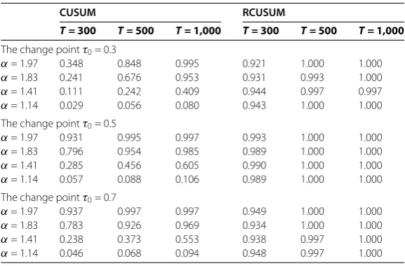
Now we shall show the power of the two tests through empirical powers. The empirical powers are calculated based on the rejection numbers of the null hypothesisHin , repetitions when the alternative hypothesisHholds. The results are included in Tables , , , . On the basis of Tables , , , , we can draw some conclusions. (i) The two CUSUM tests based on the Bartlett kernel and the quadratic spectral kernel become more powerful as the sample size T becomes larger. (ii) As the tail of the innovations gets heavier, the ordinary CUSUM test becomes less powerful, especially, the test hardly works, while the CUSUM test based on indicators is rather robust to the heavy-tailed innovations. (iii) The selection of the bandwidth has lower impact on the powers of the two CUSUM tests.

Finally, we consider the eﬀects of the skewness in the innovations{et}on the power of

[image:5.595.151.442.298.431.2]

(6)

[image:6.595.152.441.106.294.2]

Table 3 The empirical powers of the robust CUSUM test and the CUSUM test for dependent innovations

T = 300 T = 500 T = 1,000 T = 300 T = 500 T = 1,000

The change pointτ0= 0.3

α= 1.97 0.849 0.991 0.998 0.951 0.999 1.000 α= 1.83 0.692 0.919 0.977 0.964 1.000 1.000 α= 1.41 0.222 0.361 0.530 0.957 0.995 1.000 α= 1.14 0.047 0.065 0.076 0.964 0.998 1.000 The change pointτ0= 0.5

α= 1.97 0.972 0.995 0.999 0.958 0.999 1.000 α= 1.83 0.875 0.944 0.978 0.962 0.997 1.000 α= 1.41 0.300 0.446 0.542 0.964 0.999 1.000 α= 1.14 0.063 0.080 0.104 0.972 1.000 1.000

The values in Table 3 are based on the Bartlett kernel and the bandwidthγT= [4(T/100)1/4].

T = 300 T = 500 T = 1,000 T = 300 T = 500 T = 1,000

α= 1.97 0.937 0.997 0.997 0.949 1.000 1.000 α= 1.83 0.783 0.926 0.969 0.934 1.000 1.000 α= 1.41 0.238 0.373 0.553 0.938 0.997 1.000 α= 1.14 0.046 0.068 0.094 0.948 0.997 1.000

The values in Table 4 are based on the Bartlett kernel and the bandwidthγT= [8(T/100)1/4].

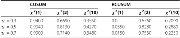
,  and , respectively. On the basis of the simulations, the skewness of the innovations aﬀects the powers the two CUSUM test signiﬁcantly.

4.2 Empirical application

[image:6.595.152.441.351.541.2]

(7)

[image:7.595.152.441.105.294.2]

T = 300 T = 500 T = 1,000 T = 300 T = 500 T = 1,000

α= 1.97 0.993 1.000 1.000 0.873 0.961 0.996 α= 1.83 0.736 0.773 0.845 0.820 0.947 0.999 α= 1.41 0.736 0.773 0.845 0.717 0.867 0.972 α= 1.14 0.570 0.556 0.594 0.577 0.731 0.878

[image:7.595.152.440.354.543.2]

The values in Table 5 are based on the quadratic spectral kernel and the bandwidthγT= [4(T/100)1/4].

T = 300 T = 500 T = 1,000 T = 300 T = 500 T = 1,000

α= 1.97 0.992 1.000 1.000 0.782 0.924 0.997 α= 1.83 0.974 0.981 0.992 0.802 0.924 0.990 α= 1.41 0.749 0.800 0.881 0.604 0.756 0.942 α= 1.14 0.544 0.580 0.590 0.448 0.598 0.838

The values in Table 6 are based on the quadratic spectral kernel and the bandwidthγT= [8(T/100)1/4].

Table 7 The empirical powers of the two CUSUM test for the skewed dependent innovations

χ2(1) χ2(2) χ2(10) χ2(1) χ2(2) χ2(10) τ0= 0.3 0.9400 0.6690 0.3550 0.0 0.6760 0.2090

τ0= 0.5 0.9940 0.8130 0.4270 0.0350 0.8280 0.2880

τ0= 0.7 0.9900 0.7140 0.3480 0.0150 0.7530 0.2250

[image:7.595.151.441.595.657.2]

(8)

[image:8.595.119.479.77.518.2] [image:8.595.116.477.80.281.2]

Figure 1 Stock prices of LBC in Shanghai Stock Exchange.

Figure 2 The logarithm return rates of LBC in Shanghai Stock Exchange.

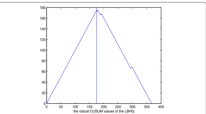
Fitting a mean and computing the test proposed in this paper= . > ., which indicates that a change in mean occurred, andT(k) attains its maximum atk=  (st, March, ) (as shown in Figure ). Recall that LBC issued an announcement that its net profits in  would decrease to % of that in , in the rd Session Board of Directors’ th Meeting on March th,  (k= ). The influence of the bad news was so strong that the stock price fell immediately in the following nine days, the mean of the logarithm return rate has a significant change afterk= .

5 Concluding remarks

(9)

[image:9.595.121.477.79.276.2]

Figure 3 The robust CUSUM values of LBC in Shanghai Stock Exchange.

of an autoregressive model is not assumed to be known a priori and has to be estimated. Second, the often-used way to determine the order via the Akaike information criterion (AIC) and the Bayes information criterion (BIC) tends to overestimate its order if a change exists. However, the proposed test does not rely on the precise autoregressive models and the prior knowledge on the tail indexα, so the proposed test is more applicable, although there exists a little distortion in its size for dependent sequences.

Appendix: Proofs of main results

The proof of Theorem  is based on the following four lemmas.

Lemma  For Lr-bounded strong(α-)mixing random variables yTt∈R,for which the mix-ing coeﬃcients satisfyα(m)≤Cm–r/(r–)–η_{for some}_η_{> ,}

E max ≤i≤T

_i

t=

(yTt–EyTt)

 ≤C

T

t=

yTt_r ()

for constants C and C,whereX= (E|X|r₎/r_.

This lemma is Lemma  in De Jonget al.[]; it is crucial for the proof of the following lemmas and theorems.

Lemma  Let

yj(φ) =sgnYj–μ–μ˜–φT–/

–sgn(Yj–μ–μ˜). ()

If the null hypothesis Hholds,then under Assumption,for all K,ε> ,

lim

δ→lim sup_T_→∞ P

sup

φ,φ∈[–K,K]:|φ–φ|<δ

T–/ T

t=

yj(φ) –yjφ–Eyj(φ) +Eyjφ >ε

= .

(10)

Proof Since the proof is similar to Lemma  of De Jonget al.[], we omit it.

Lemma  Let yj(φ)be as in(),and let

GT(τ,φ) =T–/

[Tτ]

j=

yj(φ). ()

If the null hypothesis Hholds,then under Assumption,for any K> ,

sup

τ∈[,] sup

φ∈[–K,K]

_GT(τ,φ) –EGT(τ,φ) →P . ()

Proof The proof is similar to Lemma  of De Jonget al.[], so we omit it.

Lemma  If the null hypothesis Hholds,then under Assumption,

T/(mT–μ–μ˜) = –f()–σWT() +oP(). ()

Proof The proof is similar to Lemma  of De Jonget al.[], so we omit it.

Proof of Theorem According to Lemma , we can ﬁnd a largeKso that –K≤T/(mT–

μ–μ˜)≤K. Then

T–/ST,[Tτ]=T–/ [Tτ]

j=

sgn(Yj–mT) =T–/

[Tτ]

j=

sgn(Yj–μ–μ˜) – (mT–μ–μ˜)

=GT

τ,T/(mT–μ–μ˜)

–EGT

τ,T/(mT–μ–μ˜)

+T–/

[Tτ]

j=

sgn(Yj–μ–μ˜) – T–/[Tτ](mT–μ–μ˜)f(mT˜ –μ–μ˜)

=I+I–I, ()

wheremT˜ is on the line betweenmTandμ+μ˜andmT˜ –μ–μ˜=oP() by Lemma . Then

I=oP() holds uniformly for allτ ∈[, ] by Lemmas , . By deﬁnition,I=σWT(τ). I=τ σWT() +oP() by Lemma . So we have

T–/ST,[Tτ]=σ

WT(τ) –τWT()

+oP(). ()

Noting that|T–/T

j=sgn(Yj–mT)| ≤T–/, we have

 √

TST,[T(–τ)]=T

–/

T

j=[Tτ]+

sgn(Yj–mT)

=T–/ T

j=

sgn(Yj–mT) –T–/

[Tτ]

j=

sgn(Yj–mT)

=OT–/–

GTτ,T/(mT–μ–μ˜)

–EGTτ,T/(mT–μ–μ˜)

(11)

+T–/

[Tτ]

j=

sgn(Yj–μ–μ˜)

– T–/[Tτ](mT–μ–μ˜)f(m˜T–μ–μ˜)

=OT–/–oP() –σWT(τ) –τ σWT(). ()

Based on (), (), by the functional central limit theorem,

T/σ–max

τ∈(,)|T| ⇒ _τ∈sup_(,)

_W₍τ) –τW() , asT→ ∞. ()

If we can showσˆ→P σ, the proof of Theorem  is completed. Under the null hypothesis

H,μremains as a constant, so we can prove the consistency ofσˆjust as De Jonget al.

[].

The proof of Theorem  is based on Lemmas , , ,  as follows.

Lemma  If the alternative hypothesis Hholds and k= [Tτ]is the change point,let yj(φ) be as follows:

yj(φ) =sgnYj–μ∗–φT–/–sgnYj–μ∗, ()

then under Assumption,for all K,ε> ,

lim

δ→lim sup_T_→∞ P

sup

φ,φ∈[–K,K]:|φ–φ|<δ

T–/ T

j=

= .

()

Proof Foryj(φ) as in (), we have

Eyj(φ) =

F(μ∗–μ) – F(μ∗+φT–/–μ), j≤k,

F(μ∗–μ) – F(μ∗+φT–/–μ), t>k. ()

Then forT large enough such thatKT–/_≤_η_{, under the alternative hypothesis}_H_,

sup

φ,φ:|φ–φ|<δ

T–/ T

j=

Eyj(φ) –Eyjφ

≤ sup

φ,φ:|φ–φ|<δ

T–/ k

j=

Eyj(φ) –Eyjφ + sup

φ,φ:|φ–φ|<δ

T–/ T

j=k+

Eyj(φ) –Eyjφ

=I+I, ()

I=  sup

φ,φ:|φ–φ|<δ

T–/ k

j=

(12)

=  sup

φ,φ:|φ–φ|<δ

T–/ k

j=

Fμ∗+φT–/–μ

–Fμ∗+φT–/–μ

≤ sup

φ,φ:|φ–φ|<δ

T–/ k

j= sup x∈[–η,η]

f(x)T–/ φ–φ ≤δ sup x∈[–η,η]

f(x), ()

I=  sup

φ,φ:|φ–φ|<δ

T–/ T

j=k+

Eyj(φ) –Eyj

φ

=  sup

φ,φ:|φ–φ|<δ

T–/ T

j=k+

Fμ∗+φT–/–μ

–Fμ∗+φT–/–μ

≤ sup

φ,φ:|φ–φ|<δ

T–/ T

j=k+

sup x∈[–η,η]

f(x)T–/ φ–φ ≤δ sup x∈[–η,η]

f(x), ()

whereηstands for diﬀerent constants at diﬀerent equations. This establishes equiconti-nuity ofIandI. Similar to (), we have

sup

φ,φ∈[–K,K]:|φ–φ|<δ

T–/ T

j=

yj(φ) –yj

φ

≤ sup

φ,φ∈[–K,K]:|φ–φ|<δ

T–/ k

j=

yj(φ) –yjφ

+ sup

φ,φ∈[–K,K]:|φ–φ|<δ

T–/ T

j=k+

yj(φ) –yjφ

=I+I. ()

Sinceyj(φ) is non-increasing inφ,

I= sup

φ,φ∈[–K,K]:|φ–φ|<δ

T–/ k

j=

yj(φ) –yjφ

= sup

–[K/δ]–≤i≤[K/δ]

sup

φ,φ∈[–K,K]∩[iδ,(i+)δ]

T–/ k

j=

yj(φ) –yjφ

≤ sup –[K/δ]–≤i≤[K/δ]

T–/ k

j=

yj(iδ) –yj(i+ )δ

=oP() + sup

–[K/δ]–≤i≤[K/δ]

T–/ k

j=

E yj(iδ) –yj

(i+ )δ

≤oP() + sup

φ,φ∈[–K,K]:|φ–φ|<δ

T–/ k

j=

E yj(φ) –yj

φ , ()

and the last term has been proved earlier to be equicontinuous. Similarlyyj(φ) is

(13)

I= sup

φ,φ∈[–K,K]:|φ–φ|<δ

T–/ T

j=k+

yj(φ) –yjφ

= sup

–[K/δ]–≤i≤[K/δ]

sup

φ,φ∈[–K,K]∩[iδ,(i+)δ]

T–/ T

j=k+

yj(φ) –yjφ

≤ sup –[K/δ]–≤i≤[K/δ]

T–/ T

j=k+

yj(iδ) –yj(i+ )δ

=oP() + sup

–[K/δ]–≤i≤[K/δ]

T–/ k

j=

E yj(iδ) –yj

(i+ )δ

≤oP() + sup

φ,φ∈[–K,K]:|φ–φ|<δ

T–/ T

j=k+

E yj(φ) –yjφ , ()

and the last term has been proved earlier to be equicontinuous too. By the triangle in-equality, for allε> ,

P

sup

φ,φ∈[–K,K]:|φ–φ|<δ

T–/ T

j=

≤P

sup

φ,φ∈[–K,K]:|φ–φ|<δ

T–/ k

j=

yj(φ) –yjφ–Eyj(φ) +Eyjφ >ε/

+P

sup

φ,φ∈[–K,K]:|φ–φ|<δ

T–/

T

j=k+

yj(φ) –yj

φ–Eyj(φ) +Eyj

φ >ε/

=I+I, ()

I=P

sup

φ,φ∈[–K,K]:|φ–φ|<δ

T–/ k

j=

yj(φ) –yj

φ–Eyj(φ) +Eyj

φ >ε/

≤P

sup

φ,φ∈[–K,K]:|φ–φ|<δ

T–/ k

j=

yj(φ) –yjφ >ε/

+P

sup

φ,φ∈[–K,K]:|φ–φ|<δ

T–/ k

j=

Eyj(φ) –Eyjφ >ε/

≤oP() +P

sup

φ,φ∈[–K,K]:|φ–φ|<δ

T–/ k

j=

, ()

the last term converges to  asδ→ by the equicontinuity of (). Similarly, we can show

I =P

sup

φ,φ∈[–K,K]:|φ–φ|<δ

T–/ T

j=k+

yj(φ) –yjφ–Eyj(φ) +Eyjφ >ε/

≤P

sup

φ,φ∈[–K,K]:|φ–φ|<δ

T–/ T

j=k+

yj(φ) –yj

φ >ε/

(14)

+I

sup

φ,φ∈[–K,K]:|φ–φ|<δ

T–/ T

j=k+

≤oP() +P

sup

φ,φ∈[–K,K]:|φ–φ|<δ

T–/ T

j=k+

, ()

the last term converges to  as δ→ by the equicontinuity of () too. Now, we have

completed the proof of Lemma .

Lemma  If the alternative hypothesis Hholds,let yj(φ)be as in(),and

GT(τ,φ) =T–/

[Tτ]

j=

yj(φ), ()

then under Assumption,for any K> ,

sup

τ∈[,] sup

φ∈[–K,K]

GT(τ,φ) –EGT(τ,φ) →P . ()

Proof Just as De Jonget al.[], we can obtain from Kim and Pollard [, Theorem .]

sup

τ∈[,] sup

φ∈[–K,K]

GT(τ,φ) –EGT(τ,φ) →P  ()

through the arguments for the ﬁnite-dimensional convergence for eachφ∈[–K,K] and the stochastic equicontinuity ofsup_τ_∈_[,]|GT(τ,φ) –EGT(τ,φ)|. For everyφ∈[–K,K], by Lemma , forT large enough such thatKT–/_≤_η_{, we have}

E sup

τ∈[,]

GT(τ,φ) –EGT(τ,φ)



≤CT– T

j=

sgnYj–μ∗–φT–/–sgnYj–μ∗ r

=CT– k

j=

sgnXj+μ–μ∗–φT–/

–sgnXj+μ–μ∗ 

r

+CT– T

j=k+

sgnXj+μ–μ∗–φT–/

–sgnXj+μ–μ∗ 

r

≤Cτ F

μ∗–μ+KT–/

–Fμ∗–μ–KT–/ /r

+C( –τ) Fμ∗–μ+KT–/

–Fμ∗–μ–KT–/ /r

≤C τ

sup x∈[–η,η]

f(x)KT–/ /r

+C ( –τ)

sup x∈[–η,η]

f(x)KT–/ /r

(15)

where constantsC,C,C > . Now we have shown the ﬁnite-dimensional convergence for eachφ∈[–K,K]. By the triangle inequality,

_sup τ∈[,]

_GT(τ,φ) –EGT(τ,φ) – sup

τ∈[,]

_GT

τ,φ–EGTτ,φ

≤ sup

τ∈[,]

GT(τ,φ) –EGT(τ,φ) –GT

τ,φ+EGT

τ,φ

≤T–/ T

j=

yj(φ) –yjφ–Eyj(φ) +Eyjφ . ()

Now stochastic equicontinuity follows from Lemma .

Lemma  If the alternative hypothesis Hholds,then under Assumption,

T/mT–μ∗=OP(), ()

whereμ∗is deﬁned as the median of().

Proof ForTlarge enough such thatT≥K_η–_,

sup

φ>K T–/

T

j=

sgnYj–μ∗–φT–/

≤T–/ T

j=

sgnYj–μ∗–KT–/

=T–/ k

j=

sgnXj+μ–μ∗–KT–/

+T–/ T

j=k+

sgnXj+μ–μ∗–KT–/

≤oP() +T–/ k

j=

 – FKT–/+μ∗–μ

+oP() +T–/ T

j=k+

 – FKT–/₊_μ∗_–_μ 

=oP() +T/ – F∗μ∗+KT–/

=oP() – K inf –η<(x–μ∗)<ηf

∗₍_x_), _()

which implies that lim sup_T_→∞P(T/(mT–μ∗) >K) can be made arbitrarily small by choosingKlarge enough under the alternative hypothesisH. ForP(T/(mT–μ∗) < –K),

a similar result can be derived, which proves thatmT–μ∗=OP(T–/) under the

alterna-tive hypothesisH.

(16)

T–/₍_mT_–_μ∗₎_≤_K_{will happen with arbitrarily large probability. Then}

T–ST,[Tτ]=T– [Tτ]

j=

sgn(Yj–mT)

=T–

[Tτ]

j=

sgnXj+μ–μ∗

–mT–μ∗

+T–

[Tτ]

j=[Tτ]+

sgnXj+μ–μ∗

–mT–μ∗

=T–/GTτ,T/mT–μ∗–EGTτ,T/mT–μ∗

+T–

[Tτ]

j=

sgnYj–μ∗

+T–/EGT

τ,T/mT–μ∗

=I+I+I. ()

ThenI=oP() by Lemma ,I=oP() by (), with Proposition . of Fan and Yao [],

we have

T–ST,[Tτ]

P

→τF

μ∗–μ

+ (τ–τ)Fμ∗–μ

.

Similarly, we can obtain

T–S_T_,[_Tτ] = T–

T

j=[Tτ]+

sgn(Yj–mT)

P

→( –τ)Fμ∗–μ

. ()

By the deﬁnition ofT(τ),

T(τ) P

→( –τ)τ F

μ∗–μ

–Fμ∗–μ ()

asT→ ∞, andτ≥τ, so

sup

τ∈(,)

T(τ) P

→τ( –τ) F

μ∗–μ

–Fμ∗–μ . ()

Proof of Theorem Under the hypothesisH, there is no shift in the mean, so the proof of (i) is nearly similar to the proof of the consistency ofσˆT, so we just gave the details of

the proof of (ii).

Noting that foryjdeﬁned in (),

sgn(Yj–mT) =

yj

T/mT–μ∗

–Eyj

T/mT–μ∗

+EyjT/mT–μ∗+sgnYj–μ∗

(17)

so

ˆ

σ=T– T i= T j=

k(i–j)/γT

(aTi+bTi+ci)(aTj+bTj+cj). ()

Under the assumption thatγT→ ∞,γT/T →,γT/T→ asT→ ∞, foryj(φ) deﬁned

in (), by Lemma , we havebTi=OP(T–/), then

T– T i= T j=

k(i–j)/γT

bTiaTj≤T–/ T

j= |aTj|

T

t=–T

k(t/γT)×OP() =OP(γT/T),

T– T i= T j=

k(i–j)/γT

bTibTj≤CT– T i= T j=

k(i–j)/γT

=OP

T–γT , and that T– T i= T j=

k(i–j)/γT

bTicj≤T–/ T j= cj T i=

k(i–j)/γT

×OP()

and E T–/ T j= cj T s=

k(j–s)/γT 

≤CT– T j= ct T s=

k(j–s)/γT



r

≤CT– T j= _T s=

k(j–s)/γT 

≤C T– T

j=

_T

t=–T k(t/γT)



≤C T–γ_T.

Therefore under Assumption  and the alternative hypothesis H, σˆ _{is asymptotically} equivalent to T– T t= T s=

k(t–s)/γT

(aTt+cs)(aTs+cs).

Furthermore, T– T t= T s=

k(t–s)/γT aTtcs = ∞ –∞ T– T t= T s=

aTtcsexpiξ(t–s)

ψ(ξ)dξ

≤T–/ T

t= |aTt|

∞ –∞ T–/ T s=

csexp(–isξ/γT)

(18)

andT–/T

t=|aTt|=oP() by Lemma  under Assumption , and the second term isOP() because

E ∞

–∞

T–/

T

s=

csexp(–isξ/γT)

ψ(ξ)dξ

≤

∞

–∞

ψ(ξ) dξsup

ξ∈R T–/

T

s=

csexp(–isξ/γT)

 <∞.

Finally,

T–

T

t=

T

s=

k(t–s)/γT

aTtaTs≤

∞

–∞

ψ(ξ) dξ

T–/

T

t= |aTt|



by the last term isoP() by Lemma  and Assumptions , , so we have shown thatσˆ

asymptotically equals

T– T

i=

T

j=

k(i–j)/γT

cicj. ()

Under Assumptions ,  and the alternative hypothesisH,{sgn(Yj–μ∗)}satisﬁes the as-sumptions of Theorem . in De Jong and Davidson [], so

T– T

i=

T

j=

k(i–j)/γT

cicj→P σ_, ()

so the proof of Theorem  has been completed.

Competing interests

The authors declare that they have no competing interests.

Authors’ contributions

All authors contributed equally to the writing of this paper. All authors read and approved the ﬁnal manuscript.

Author details

1_{School of Mathematical Science, Shanxi University, Taiyuan, Shanxi 030006, P.R. China.}2_{Institute of Management and} Decision, Shanxi University, Taiyuan, Shanxi 030006, P.R. China.

Acknowledgements

The authors are grateful to the two anonymous referees for their careful reading of the manuscript and many helpful comments which improve the manuscript greatly. We would like to thank Prof. John Nolan who provided the software for generating the stable innovations in Section 4. By ﬁnancial support this work is supported by the National Natural Science Foundation of China (No. 11226217) and the Postdoctoral Science Special Foundation (Nos. 2012M510772, 2013T60266), which is gratefully acknowledged.

Received: 12 May 2014 Accepted: 19 January 2015 References

1. Sen, A, Srivastava, MS: On tests for detecting change in mean. Ann. Stat.3, 96-103 (1975)

2. Hawkins, DM: Testing a sequence of observations for a shift in location. J. Am. Stat. Assoc.72, 180-186 (1977) 3. Worsley, KJ: On the likelihood ratio test for a shift in locations of normal populations. J. Am. Stat. Assoc.74, 365-367

(1979)

4. Yao, YC: Approximating the distribution of the ML estimate of the change point in a sequence of independent random variables. Ann. Stat.3, 1321-1328 (1987)

(19)

6. Horváth, L, Kokoszka, P: The eﬀect of long-range dependence on change-point estimators. J. Stat. Plan. Inference64, 57-81 (1997)

7. Mittnik, S, Rachev, S: Stable Paretian Models in Finance. Wiley, New York (2000)

8. Phillips, PCB: Time series regression with a unit root and inﬁnite-variance errors. Econom. Theory6, 44-62 (1990) 9. Horváth, L, Kokoszka, P: A bootstrap approximation to a unit root test statistics for heavy-tailed observations. Stat.

Probab. Lett.62, 163-173 (2003)

10. Han, S, Tian, Z: Truncating estimator for the mean change-point in heavy-tailed dependent observations. Commun. Stat., Theory Methods35, 43-52 (2006)

11. Han, S, Tian, Z: Bootstrap testing for changes in persistence with heavy-tailed innovations. Commun. Stat., Theory Methods36, 2289-2299 (2007)

12. Hušková, M: Tests and estimators for change point problem based onM-statistics. Stat. Decis.14, 115-136 (1996) 13. Hušková, M:M-Procedures for detection of changes for dependent observations. Commun. Stat., Simul. Comput.41,

1032-1050 (2012)

14. De Jong, RM, Amsler, C, Schimidt, P: A robust version of the kpss test based on indicators. J. Econom.137, 311-333 (2007)

15. Wang, JH, Wang, YL, Ke, AM: The stable distributions ﬁtting and testing in stock returns of China. J. Wuhan Univ. Technol.25, 99-102 (2003)

16. Kim, J, Pollard, D: Cube root asymptotics. Ann. Stat.18, 191-219 (1990)

17. Fan, J, Yao, Q: Nonlinear Time Series: Nonparametric and Parametric Methods. Springer, Berlin (2003) 18. De Jong, RM, Davidson, J: Consistency of kernel estimators of heteroscedastic and autocorrelated covariance