A fault simulation methodology for MEMS

A Fault Simulation Methodology for MEMS

R. Rosing, A.M. Richardson & A.P. Dorey

Microsystems Research Group, Lancaster University, Lancaster LA1 4YR, UK.

Abstract

Efficient built-in and external test strategies are becoming essential in MicroElectroMechanical Systems (MEMS), especially for high reliability and safety critical applications. To be realistic however, internal and external test must be properly validated in terms of fault coverage. Fault simulation is hence likely to become a critical utility within the design flow.

This paper will discuss methods for achieving test support based on the extension of tools and techniques currently being introduced into the mixed signal ASIC market.

1.

Introduction

Both current and expected applications of MEMS tend to be in sensing and actuation where, in many cases, the device will play a mission critical role. Examples here are pressure sensors for aircraft engine control, vehicle braking, vessel pressure in reactors and medical implants. These devices will also tend to have mechatronic interfaces or at the least, non-electrical inputs and limited access for test. High quality production test, self-test and on-line data validation are all likely to become critical specifications for these devices.

To support fault simulation and testability analysis in MEMS, it is necessary to model both the mechatronic and electrical elements within the same simulation environment to ensure the efficient injection and analysis of faults. In most cases, the fault simulation process must be carried out in closed loop configuration to allow non-idealities that can effect fault coverage such as process variations, noise, mode coupling and resolution limitations to be handled correctly.

This paper proposes methods of extending the capabilities of mixed signal and analogue fault simulation techniques to MEMS by including failure mode and effect analysis data and using behavioural modelling techniques compatible with electrical simulators. The methodology is based on preliminary work [1] and builds on component level modelling used in design and test studies at both Robert Bosch GmbH [2,3] and Carnegie Mellon University [4]. Methods of modelling both micromechanical structures and interface electronics in closed loop configuration are discussed with concepts illustrated on a silicon resonant pressure sensor.

2.

Modelling of transducers

2.1.

Lumped level modelling

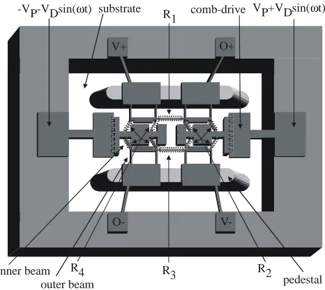
Lumped level modelling of transducers will be explained using an example industrial micromachined resonant pressure sensor [5]. An exaggerated illustration of the movement of the sensor is shown in figure 2.1.

O+

-V -V sin( t)_{P D} ω V +V sin( t)_{P D} ω

V+

O-

V-R1

R3

R4 R2

comb-drive substrate

pedestal inner beam

outer beam

Figure 2.1. Pressure sensor

In the operating mode of the system, the electrostatic forces within the comb-drives cause the two movable structures to oscillate in opposite directions. The structures therefore separate and then close. Due to the stiffness of the piezoresistors connecting the two movable parts, the movement of the outer beams is negligible compared to the movement of the inner beams.

to bend. The pedestals therefore separate and cause a tension in the beams that form the spring. This tension causes the spring stiffness and therefore the resonant frequency of the system to change.

A high-level description of this sensor has been generated in the behavioural language ABCD within the mixed signal simulator "SMASH" (marketed by Dolphin Integration). The sensor is implemented as a set of equations in a subcircuit of a system netlist. For reasons of confidentiality, the design parameters associated with the sensor have been altered.

The movable part of the structure is simply described by its’ mass. The four beams connected to each movable part are modelled as one spring. The following analytical solution is used to model the relationship between the stiffness of the beams (spring ‘constant’) and the tension in the structure:

L

5

T

6

L

EI

12

k

=

+

Where I represents the second moment of area, E Young’s modulus, L the length of the beam and T the force in the axial direction (caused by the bending of the substrate). This relationship differs from a finite element relationship in that the spring stiffness has no longer a constant value.

An equivalent mass of the beams is calculated and added to the mass of the movable part.

Derivation of the relationship between the measurement pressure and the tension in the springs is currently being carried out. The results of finite element simulations on the membrane with pedestals will be used to derive this relationship.

An analytical solution is used to model the relationship between the applied drive voltage and the electrostatic force. The electrical behaviour of the comb-drive has been modelled as a varying capacitance as a function of movement.

The piezoresistors R4 and R2 (both consisting of four resistors) will not change value during movement, since the effect of part of each resistor being compressed is cancelled out by the other part being extended. The piezoresistors R1 and R3 change value with a frequency equal to the resonance frequency of the structure. The applied force to and the relative change of resistance value of these piezoresistors are related by the piezoresistance

coefficient, π. From figure 2.1 it can be seen that the

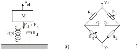
piezoresistors form a Wheatstone bridge, as is schematically modelled in figure 2.2.b. The output (O+ -O-) of this bridge is the sum of a sine wave voltage at the resonance frequency and a bias voltage.

In [6], damping in laterally driven microresonators is derived based on Stokes flow and Couette flow. Analytical solutions are found to match experimental results for

resonators operating at atmospheric pressure. For systems operating at very low pressures, the viscosity of the ambient gas is not well defined and it becomes more difficult to derive the damping. Furthermore, damping mechanisms in the material may not in this case be negligible. Further research has to be applied in this field.

M

k(p) _Rd

Fel

F + F_{d k}

a)

O- O+ V+

V-R4 R1

R3 R2

b)

Figure 2.2. Lumped modelling of the sensor

This example illustrates that lumped modelling of transducers is similar to behavioural modelling of electrical circuit blocks. In both cases only the functionality of the circuit is described. The elements of which the circuit is constructed are not individually modelled (all the beams in the sensor are modelled as one stiffness value).

2.2.

Component level modelling

The description of sensors and actuators at a component level is based on the fact that these structures can be described as an interconnected set of elements. A microelectromechanical structure can for example be described as being implemented from elements such as masses and beams. When behavioural descriptions are generated for those elements, the structure can be modelled at a schematic level. This is similar to an electrical schematic, which consists of a number of electrical components, for which behavioural descriptions (for example the equations modelling a transistor) are derived.

To form a component level description of the entire transducer, the behavioural models of the separate components have to be linked using "through" and "across" variables. In the electrical domain these variables correspond to currents and voltages respectively. Kirchhoff’s current law states that on each node of the schematic, the sum of currents equals zero. In a closed-loop within the schematic the sum of voltages equals zero (Kirchoff’s Voltage Law). These relationships hold in general for the corresponding through and across variables. For mechanical structures the through variables are the forces and the across variables are the displacements.

In [4] a simulator, referred to as a nodal simulator, in which transducers can be simulated at a component level, is described. Every beam of the design is described as one element characterised by its’ stiffness matrix and an effective mass matrix. The simulator can therefore be regarded as a finite element simulator in which every component is modelled by just one element.

This type of (linear) simulation will give good results for small displacements. Furthermore, on each component, the relationships between forces and displacements in the different directions should be approximately independent. If these demands do not hold, either non-linear analytical solutions have to be used or the results from low-level finite element simulations have to be mapped into the behavioural model.

Modelling of beam elements is described in [3]. The natural frequencies of the beams are simulated by splitting the beam into more than one element. In [2] a microgyroscope system is modelled. Finite element simulations are used to derive descriptions of components for which it is difficult to find an analytical solution.

2.3.

Closed loop system simulation

A behavioural level description or a schematic level description of the sensor/actuator can be implemented in an electrical simulator, which either incorporates or can be used in combination with a behavioural language supporting the use of non-electrical variables. This enables the combined simulation of electrical circuitry and the

sensor/actuator and therefore microsystem fault

simulation. Examples of programs that enable these simulations are the combination of ELDO (a mixed-signal

simulator marketed by Mentor Graphics®) and

VHDL-AMS, SABER (a mixed-signal simulator marketed by Analogy Inc.) with its’ behavioural language MAST and SMASH with its’ behavioural language ABCD. Examples of tools that support hierarchical fault simulation are MiST PROFIT [7], Faultmaxx [8] and GDSFaultsim [9]. Some of these tools combine hierarchical and statistical fault simulation.

A possible realisation of the pressure sensor within a closed loop with electrical circuitry is shown in figure 2.3. As with the sensor, behavioural models of the electrical circuit blocks have been implemented in subcircuits within SMASH. The system is therefore modelled at the highest level of abstraction of a hierarchical system (that is: all blocks are behavioural).

Depending on the pressure of the surrounding atmosphere, the quality factor of this sensor can vary between 1600 (at atmospheric pressure) to over 40.000 (in a high vacuum). A sensor with a larger quality factor will lead to a slower response and will increase the accuracy demands on the simulator. The simulation time therefore increases with quality factor. Quality factors of MEM transducers in high vacuum are orders of magnitude higher

than typical quality factors in electrical circuits. Problems with convergence can therefore occur.

In this case a quality factor of 2000 has been used in the simulation models of the sensor. A resonant frequency of 53 kHz is realistic for this system.

Sensor

Differential Amplifier

Low-pass filter

90 phase shift

o

fout -1

Rectifier Smoother VHP

Vsmooth VAGC AGC

O+

O

-Vin,sens _R1 R2

Figure 2.3. Block diagram of the closed-loop system

The output voltage of the smoothing circuit, Vsmooth,

determines the resistance between the drain and the source of the MOSFET. The gain of the inverting amplifier circuit is therefore given by:

(

)

2

V

R

R

gain

=

Noise in the system blocks will cause the sensor to start oscillating. The oscillation will build up to the required amplitude (chosen by the designer) when a decreasing amplitude of the output signal of the sensor (caused by damping) leads to an increasing amplitude of the signal fed back into its input pads from the AGC. At the required amplitude the closed-loop gain should equal 1. For reasons of brevity the complete derivation of the operating condition is not shown here.

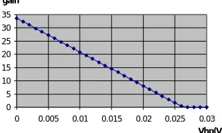
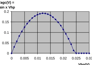
In figures 2.4 and 2.5 both the gain and the amplitude of the output signal of the automatic gain control are plotted versus the output amplitude of the capacitor output node (functioning as a high-pass filter).

0 5 10 15 20 25 30 35

0 0.005 0.01 0.015 0.02 0.025 0.03

Vhp(V) gain

Figure 2.4. Gain versus input AGC

For input signal amplitudes (Vhp), larger than 12.5mv,

0 0.05 0.1 0.15 0.2 0.25

0 0.005 0.01 0.015 0.02 0.025 0.03

Vhp(V)

Vagc(V)=gain x Vhp

Figure 2.5. Output versus input AGC

A Vhp of 18mV puts the system at the correct operating

point. The phase shift circuit is implemented as two RC networks connected in series, both with their cut-off frequency equal to the resonance frequency of the sensor

(and therefore generating a 450 phase shift). The 200mV

output signal is attenuated by the phase shifter and results in a 100mV input signal to the sensor, which is required to obtain a closed-loop gain of 1. Application of a sinusoidal voltage with amplitude of 100mV on top of a bias voltage of 50V to the input of the sensor in an open-loop configuration, shows that this results in an output signal from the high-pass filter of approximately 18mV. This can be seen in figure 2.6.

20nV 16nV 12nV 8nV 24nV

4nV 0V -4nV -8nV -12nV -16nV -20nV 20mV 16mV 8mV 4mV 0V -4mV -8mV -12mV -16mV -20mV 10m 20m 30m 40m 50m 60m 70m 80m 90m Scaling: V(XB1.Y)

V(HP)

12mV

Figure 2.6. Sinewave response

In figure 2.6, the signal XB1.Y (signal Y in subcircuit XB1) represents the displacement of one of the movable parts of the resonator.

Due to the low damping of the system the oscillation takes a large number of cycles to build up. Therefore, only the envelope of the signals is visible.

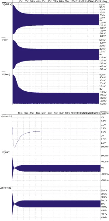
The loop is now closed and a piecewise linear voltage source is used to simulate a ‘pulse’. This pulse is applied to the input of the sensor together with the bias voltage and the feedback signal. The impulse response of the

closed-loop system is shown in figure 2.7.The rectifier is

implemented as a simple mathematical function, ensuring that the output signal is equal to the absolute value of its input signal.

V(XB1.Y)

V(HP)

V(Rect)

10m 20m 30m 40m 50m 60m 70m 80m 90m 110m 130m140m 50nV 40nV 30nV 20nV 10nV 0V -10nV -20nV -30nV -40nV -50nV -60nV 60nV

50mV 40mV 30mV 20mV 10mV Scaling:

20mV 10mV 0V -10mV -20mV -30mV -40mV -50mV 0V -10mV -20mV -30mV -40mV -50mV 50mV 40mV 30mV

Scaling: 10m 20m 30m 40m 50m 60m 70m 80m 90m 110m 130m140m V(smooth)

3.6V 3.2V 2.8V 2.4V 2V 1.6V 1.2V 800mV 4V

50.4V 50.3V 50.2V 50.1V 50V 49.9V 49.8V 49.7V 49.6V 800mV

400mV

0V -400mV

-800mV

V(FEEDB) V(AGC)

Figure 2.7. Impulse response of the closed-loop system

In the first 5ms, the capacitor in the smoother, implemented as a simple RC filter, needs to be charged. Following this, the decreasing sensor signal causes the amplitude of the smoothed signal and therefore the feedback signal to increase until the operating point is reached. In this case the system reaches its operating point, since the impulse was large enough to push it into the correct part of the automatic gain control characteristic. Where the noise in the system is not of sufficient amplitude to reach this correct part of the characteristic, a startup circuit has to be used.

3.1.

The FMEA

concept

FMEA+ was first proposed by Olbrich [10]. The

technique relies on integrating qualitative failure analysis and quantitative fault simulation. Failure Mode and Effect Analysis (FMEA) [11], is well accepted by the system design industries, whereas fault simulation tends to be restricted to low level components unless behavioural modelling techniques are used. To illustrate the need for the integration of the two methods, a brief analysis of the types of faults that can occur in MEMS devices reveals the following categories:

- Local defects

- Parameters out of tolerance

- Wear (especially in devices with movable parts)

- Environmental hazards

- Problems due to imperfection in the design process

(i.e. design validation poor compared to mixed-signal designs)

- Mode coupling / structure oscillation in incorrect

modes

- System level faults (for example crosstalk between

signals of different modules)

For CMOS circuits, defect-related and parametric faults are typically taken into account during a fault simulation. FMEA can be used to compile fault lists related to the remaining fault categories. The procedure involves:

1. Identification of all the functions of the system at all

levels of hierarchy (component, system block, and system) to be analysed.

2. Anticipation and description of how the parts at the

different levels of hierarchy can fail (failure mode).

3. Assumption that failures have occurred and

description of effect(s).

4. Identification of every possible fault cause for the

failure mode.

In a Failure Mode, Effect and Criticality Analysis (FMECA) [11,12] a ranking system is used to express the severity of the failure mode, its’ chance of occurrence and the likelihood of it being detected. FMECA will simply be denoted as FMEA throughout this paper.

A FMEA is ideally performed by a team of specialists involved in the design of the system. Since the analysis is performed at different levels of hierarchy, failure modes can be predicted at an early stage of the design. It will however not be possible to predict all failure modes and their effects accurately in a FMEA meeting. Furthermore, the ranking of the different faults is based on the subjective judgement of the FMEA team members.

Another disadvantage of the FMEA method is that it is not automated. The analysis can be automated using numerical simulations, expert systems [13] or causal

reasoning [14]. In all cases, information compiled from previous analysis of similar circuits is used. This reduces the time to generate a list of failure modes. However, both expert systems and causal reasoning suffer from a subjective evaluation of the effects of the failure modes. Furthermore, the methods that are used to evaluate these effects are not compatible with the numerical method used in fault simulation.

Many of the disadvantages mentioned above can be overcome when the faults predicted during an FMEA meeting are modelled within a hierarchical fault simulation of the Microsystem. This requires the modelling of these faults in a form compatible with the simulator.

3.2.

Analogue and mixed-signal fault simulation

The methodology generally used to generate the fault list for analogue and mixed-signal fault simulation is shown in figure 3.1.

Industrial failures

Specialist FMEA meeting System Mixed-signal

circuitry

Circuit blocks

Layout Defect description

and statistics

Parametric variations

Schematic level faults

Schematic

Fault-free behavioural models of circuit

blocks Faulty

behavioural models of circuit

blocks Extraction of

faults

Defect-related faults IFA

Figure 3.1. Generation of the fault list and beha-vioural models for mixed-signal circuitry in the

FMEA+ approach

The following procedures are core to the success of the methodology:

1. Inductive Fault Analysis (IFA) [15,16]. Here a fault

list based on the actual defects occurring in the layout can be obtained.

2. Parametric faults involving no change to the netlist

due to component parameter variation that may cause the system to fail its’ specifications.

3. The generation of behavioural models of the fault-free

Hierarchical fault simulation will be described in section 3.4.

3.3.

Transducer fault modelling and simulation

As described in [1], to generate a fault list and fault-free and faulty behavioural models for a transducer, a similar procedure to for mixed-signal fault simulation is feasible. This is shown in figure 3.2.

Defect descriptions and statistics

Layout of the sensor/actuator

Finite element description & simulation

Industrial failures Sensor/ actuator

IFA

Defect-related faults

Component level description of sensor/actuator

Parametric variations

Faults at the component

level

Fault-free behavioural model of sensor/actuator Description of faults

at a higher level

High-level faulty sensor descriptions

Specialist FMEA meeting System

In case of using electrical equivalent

models

Figure 3.2. Generation of the fault list and beha-vioural models for sensors/actuators in the

FMEA+ approach

The sort of defects that can occur in these kind of structures can be determined from observations of failed devices. In [17] the most typical failure mechanisms in a bulk micromachining process are identified for each technology step together with the faults & deviating parameters caused by those mechanisms.

In [18] the effect of one category of defects, particulate contaminations, is investigated by inserting them into a mesh description of the structure and performing finite element simulations using a Monte Carlo approach. For each fault the change in resonant frequency of an example resonator is observed. Since this is not a parameter of either the lumped model or the component level model, the effect on the closed-loop system behaviour can not be simulated in this example.

To be able to handle a fault in a closed-loop system simulation it has to be modelled at either the component level or the lumped level.

Since defects and parametric variations occur either within or between components, they can be modelled at the component level. Since every component in a component level description has the form of a parameterised cell, these faults can be modelled by either adapting the behavioural description of the component or adding an extra component. This has the advantage that a library of component level fault models can be generated and reused in future designs. Furthermore, the likelihood of occurrence of each fault can be predicted from the dimensions of the structure the fault is located in.

Faults that change the behaviour of the entire sensor have to be modelled at the lumped level. By way of adapting the behavioural description, a faulty lumped model can be generated.

An example of a fault that can not be modelled at the lumped level is a fault in one of the four beams connected to the plate (mass) of the pressure sensor. This can cause the stiffness of this beam to change. Due to the resulting asymmetry in the force-distribution, the structure will not only translate, but also rotate. This effect can not be modelled at the behavioural level, since the distributed nature of the spring is not taken into account at this level.

In the case where an electrical equivalent model is used as a lumped-level description of the structure, the component level faults have to be mapped to equivalent faults in the electrical domain. In [19] a HDL-A fault model library is used for this purpose.

To enable modelling of FMEA failure modes, it is necessary to categorise these failures to the level of modelling they require. The following categorisation is proposed:

- Failures that are directly linked to certain components.

- Failures that can be modelled at the lumped level.

The effect of system level faults have to be investigated. The other causes of failure mentioned in section 3.1 can be categorised.

The first category of faults contains some environmental effects and all other faults mentioned in section 3.1. The effect of extreme temperatures on the sensor operation can, for example be taken into account by modelling the relationship between temperature and the material properties of each component. Wear will also change the material properties of some components.

By describing the relationship between the failures in the first group and their effects at the component level, component level fault models are generated for failures defined during an FMEA analysis.

can be predicted from experience with failures of similar devices.

3.4.

Closed loop system fault simulation

The results of the trajectories shown in figure 3.1 and 3.2 can be used to perform a hierarchical and statistical fault simulation on the entire Microsystem. The results of this simulation identify difficult to detect faults and the possible need for design for testability or built-in self-test integration. This is shown in figure 3.3.a. In figure 3.3.b, hierarchical simulation of the system block is achieved by describing faults at either the component level or through faulty behavioural models. This system block can be either an electrical circuit block or a sensor/actuator.

Component level description of the system blocks

Fault-free behavioural models of system

blocks

Hierarchical and statistical fault

simulation of closed-loop system

High-level faulty descriptions of the system blocks

Effects on the closed-loop system behaviour

Design for Test/ Built-In Self-Test Faults at the

component level

a)

Behavioral model

of fault-free block Behavioral model of fault-free block N circuit level faults

insert faults sequentially

... ... ...

b)

Figure 3.3. Achieving DfT or BIST for Microsystems

As an illustration, the use of the closed loop model for evaluating two possible fault effects will now be demonstrated; one inside the sensor and one in the electrical circuitry.

A potential fault in the sensor, influencing all of its components, is too low a value of the vacuum in the hermetically sealed capsule covering the sensor. To simulate this fault, the damping is increased from the original value of 3 x 10-6 to 6 x 10-6 (this implies that the

quality factor is decreased from 2000 to 1000. The impulse response under these circumstances is shown in figure 3.4.

50nV 40nV 30nV 20nV 60nV

10nV 0V -10nV -20nV -30nV -40nV -50nV -60nV

800mV 600mV 400mV 200mV 1V

0V -200mV -400mV -600mV -800mV -1V V(XB1.Y)

V(AGC)

10m 20m 30m 40m 50m 60m 70m 80m 90m 110m 130m140mScaling:

Figure 3.4. SMASH simulation results : Impulse response for too low a vacuum

The increased damping causes the gain of the sensor to decrease. In this case, the closed-loop gain is smaller than one during the entire simulation period. Therefore, there is not enough drive to compensate for the damping and the oscillation terminates.

In the case where the damping is increased by a smaller amount, the operating point of the AGC would change in such a way that the gain is increased, bringing the closed-loop gain back to 1. In that case, the system still functions correctly, but with higher power consumption.

A potential fault in the electrical circuitry is an offset at the output of the rectifier. To illustrate the use of the model, approximately 200mv has been added to the output signal of the rectifier. This causes the operating point and therefore the gain of the MOSFET to change. In figure 3.5 it can be seen that the gain of the AGC is not sufficient to sustain oscillation in the closed-loop system.

0 0.05 0.1 0.15 0.2

0 0.005 0.01 0.015 0.02 0.025 0.03

Vhp(V) Vagc(V) =

gain x Vhp

The SMASH simulation indeed indicates that the oscillation resulting from an input pulse slowly terminates (results not shown here).

In the case where the offset is smaller, the system will function correctly, but at a different operating point. In this case the fault has a parametric effect.

4.

Conclusions & future work

To enable investigation of the effects of all possible

sources of faults, FMEA+, a combination of Failure Mode

and Effect Analysis (FMEA) and fault simulation, has to be used. It is shown how both approaches can be combined using fault & fault free modelling at different levels of hierarchy. Similarities in the extraction and modelling of faults in both MEM transducers and electrical circuitry is shown. It is explained how these similarities can be exploited to achieve a hierarchical fault simulation at a system level.

Furthermore, automation of the extraction of FMEA failures is proposed by way of categorisation of these

failures and use of fault libraries. An FMEA+ analysis on a

pressure sensing system is initialised by behavioural modelling of the different components of the sensor and the electronic circuit blocks in the feedback circuitry.

Further research will include a deeper investigation into the categorisation of different failures and the modelling of these failures at both the component and the lumped level. Furthermore, the lumped model of the pressure sensor will be completed by way of mapping finite element results for the membrane to generate its component level description . Application of the proposed strategies will lead to DfT and/or BIST proposals for this and other types of similar systems.

5.

Acknowledgements

This work has been partially supported by the European Union under the ESPRIT IV Basic Research Project 26354 - "ASTERIS" and the UK EPSRC "VALSIC" project no. GR/L98404. We would also like to thank Dolphin Integration for assistance in developing simulation models and John Greenwood at Druck UK for assistance in developing finite element models of the resonator.

6.

References

1. R. Rosing, A. Richardson, A. Dorey and A. Peyton, “Test

Support Strategies for MEMS”, Proceedings of the 5th

International Mixed Signal Testing Workshop, 1999, pp. 345-350.

2. D. Teegarden, G. Lorenz and R. Neul, “How to model and simulate microgyroscope systems”, IEEE Spectrum, July 1998, pp. 66-75.

3. R. Neul, U. Becker, G. Lorenz, P. Schwarz, J. Haase and S. Wunsche, “A Modelling Approach to Include Mechanical

Components into the System Simulation”, Proceedings of the DATE, 1998, pp. 510-517.

4. T. Mukherjee, G.K. Fedder and R.D. Blanton, “Hierarchical Design and Test of Integrated Microsystems”, IEEE Design & Test of Computers, vol. 16, no. 4, pp. 18-27, 1999. 5. C.J. Welham, J. Greenwood and M. Bertioli, “A Lateral

Resonant Pressure Sensor Fabricated Via Fusion Bonding, Wafer Thinning and Reactive-Ion-Etching”, Sensors and Actuators A, vol. 76, pp. 298-304, 1999.

6. X. Zhang and W.C. Tang, Viscous Air Damping in Laterally Driven Microresonators”, Sensors and Materials, Vol. 7, No. 6, pp 415-430, 1995.

7. R. Voorakaranam, S. Chakrabarti, J. Hou, A. Gomes, S. Cherubal, A. Chatterjee and W. Kao, “Hierarchical Specification-Driven Analog Fault Modeling for Efficient Fault Simulation and Diagnosis”, Proceedings of the International Test Conference, 1997, pp. 903-912.

8. N.B. Hamida, K. Saab, D. Marche and B. Kaminska,

‘FaultMaxx: A Perturbation Based Fault Modeling and Simulation for Mixed-Signal Circuits’, Asian Test Symposium (ATS '97), November 1997.

9. Y. Eben Aimine, A. Richardson, C. Descleves & K. Sommacal. "GDS FaultSim, a Mixed-Signal IC Computer-Aided-Test (CAT) Tool" Proceedings of DATE, March 1999. 10.T. Olbrich, “Design-for-Test and Built-In Self-Test for Integrated Systems”, Ph.D. Thesis, Lancaster University, Lancaster, U.K., September 1996.

11.British Standard Institute, BS5760, “Reliability of systems, equipment and components”, part 5: “Guide to failure modes, effects and criticality analysis (FMEA and FMECA)”, 1991.

12.J.B. Bowles, “The New SAE FMECA Standard”,

Proceedings of the Annual Reliability and Maintainability Symposium, 1998, pp. 48-53.

13.D.J. Russomanno, R.D. Bonnell and J.B. Bowles, “A

Blackboard Model of an Expert System for Failure Mode and Effects Analysis”, Proceedings of the Annual Reliability and Maintainability Symposium, 1992, pp. 483-490.

14.D. Bell, L. Cox, S. Jackson, P. Schaefer, “Using Causal Reasoning for Automated Failure Modes & Effects Analysis (FMEA)”, Proceedings of the Annual Reliability and Maintainability Symposium, 1992, pp. 343-353.

15.T. Olbrich, J. Perez, I. Grout, A. Richardson, C. Ferrer, “Defect-Oriented vs Schematic-Level Based Fault Simulation for Mixed-Signal ICs”, Proceedings of the ITC, 1996, pp. 511-520.

16.H. Walker, S.W. Director: “VLASIC: A Catastrophic Fault Yield Simulator for Integrated Circuits”, IEEE Transactions on CAD, 1986, vol. CAD-5 no. 4, pp. 541-556.

17.A. Castillejo, D. Veychard, S. Mir, J.M. Karam and B. Courtois, “Failure Mechanisms and Fault Classes for CMOS-Compatible Microelectro-mechanical Systems”, Proceedings of the ITC, 1998, pp. 541-550.

18.A. Kolpekwar, C. Kellen and R.D. Blanton, “MEMS Fault Model Generation using CARAMEL”, Proceedings of the ITC, 1998, pp. 557-566.