Rolling sampled parameters of ARCH and Levy stable models

Munich Personal RePEc Archive

Rolling-sampled parameters of ARCH

and Levy-stable models

Degiannakis, Stavros and Livada, Alexandra and Panas,

Epaminondas

Department of Statistics, Athens University of Economics and

Business

2008

Online at

https://mpra.ub.uni-muenchen.de/80464/

R o l l i n g - s a m p l e d p a r a m e t e r s o f A R C H a n d L e v y - s t a b l e

m o d e l s

Stavros Degiannakis, Alexandra Livada, Epaminondas Panas

Department of Statistics, Athens University of Economics and Business

A b s t r a c t

In this paper an asymmetric autoregressive conditional heteroskedasticity (ARCH) model and a Levy-stable distribution are applied to some well-known financial indices (DAX30, FTSE20,

FTSE100 and SP500), using a rolling sample of constant size, in order to investigate whether the values of the estimated parameters of the models change over time. Although, there are

changes in the estimated parameters reflecting that structural properties and trading behaviour alter over time, the ARCH model adequately forecasts the one-day-ahead volatility. A simulation study is run to investigate whether the time variant attitude holds in the case of a

generated ARCH data process revealing that even in that case the rolling-sampled parameters are time-varying.

Keywords: ARCH model, GED distribution, Leverage effect, Levy-stable distribution, Rolling sample, Spill over, Value at risk.

1 . I n t r o d u c t i o n

In the recent literature, regarding the description of the characteristics of financial markets, one can find a vast number of specifications of both ARCH and Stochastic Volatility (SV)

processes that have been considered for. However, the SV models1 are not as popular as the

ARCH processes in applied studies. The purpose of the present study is to apply an asymmetric ARCH model to some well known financial indices, using a rolling sample of

constant size, in order to observe the changes over time in the values of the estimated parameters. A thorough investigation is conducted by comparing the parameters of the

full-sampled estimated model to the parameters of the rolling sub-sample estimated models. We conclude that the values of the estimated parameters change over time, indicating a data set

that alters across time reflecting the information that financial markets reveal. The analysis is extended to simulated time series indicating that the time-varying estimated coefficients

characterize the ARCH data generating process itself.

In ARCH modelling, the distribution of stock returns has fat tails with finite or infinite

unconditional variance and time dependent conditional variance. Estimation of stable distributions is an alternative approach in modelling the unconditional distribution of returns. Thus, we adopt the estimation procedure of McCulloch (1986) and the parameters of the

Levy-stable distribution are estimated at each of a sequence of points in time, using a rolling

sample of constant size. The empirical findings suggest that the parameters of the unconditional distribution are also not constant over time.

Reviewing the relevant literature we notice absence of studies showing that although

the parameters of a well-specified model vary significantly over time, their time varying attitude

does not influence model’s forecasting ability. The main object of our study is to provide evidence that model’s parameters should be re-estimated on a frequent base in order to reflect any changes that have been occurred in the stock market and have been incorporated

in the prices of assets.

The paper is divided in six sections. Section 2 lays out the asymmetric ARCH model

that is applied in the FTSE20, DAX30, FTSE100 and SP500 stock indices. In section 3, the estimated rolling-sampled parameters of the asymmetric ARCH model are discussed. In

section 4, a simulation study examines whether the parameters are time-varying in the case of a generated ARCH process. In section 5, the unconditional distribution of returns is estimated and the phenomenon of time-variant parameters is investigated in the Levy-stable distribution.

Finally, in section 6 we summarize the main conclusions. 2 . A n a s y m m e t r i c A R C H m o d e l

A wide range of proposed ARCH models is covered in surveys such as Andersen and Bollerslev (1998), Bera and Higgins (1993), Bollerslev et al. (1992), Bollerslev et al. (1994),

1 _{The reader who is interested in SV models is referred to Barndorff-Nielsen et al. (2002), Chib et al. (1998),}

Degiannakis and Xekalaki (2004) and Poon and Granger (2003). The Nobel price award to

R.F. Engle for ARCH volatility modeling is the uncontested proof of the contribution of ARCH models in time series and econometric modelling (Diebold 2003). A plethora of studies applied

ARCH models to predict future volatility by updating the available information set at each of a sequence of points in time. Among others, Balaban and Bayar (2005) tested in 14 countries the relationship between stock market returns and their forecast volatility, Blair et al. (2001)

compared the information content of implied volatilities and intraday returns in the context of forecasting S&P100 volatility, Wei (2002) forecast China’s weekly stock market volatility and Yu (2002) predicted stock price volatility using daily New Zealand data. Angelidis et al. (2004), Degiannakis (2004), Brooks and Persand (2003) and Giot and Laurent (2003) predicted

Value-at-Risk (VaR) measures, while Degiannakis and Xekalaki (2001), Engle et al. (1997) and Noh et al. (1994) used rolling ARCH models to forecast volatility of options.

An ARCH process,



_t

 



, can be presented as

 

 

 

 





 



, ,...; , ,...; , ,...



, 1 , 0 ~ 2 1 2 1 2 1 2 . . .           t t t t t t t t t d i i t t t t g z V z E f z z

























1)

where



is a vector of unknown parameters,

f

 

.

is the density function of z_t,

g



.

is a linear or non-linear functional form and



t is a vector of predetermined variables included in

information set I at time

t

. Since very few financial time series have a constant conditional

mean of zero, an ARCH model can be presented in a regression form by letting



t be the

unpredictable component of the conditional mean



At t



t

t

A

E

y

I

y

_,



_,

|

_1





,

2)

where

y

A_,t



ln



P

A_,t

P

A_,t₁



denotes the continuously compound rate of return from time

t



1

to

t

, and

P

A,t is the asset price A at time

t

. In order to investigate the characteristics of stock

market A, we apply an ARCH model of the following form:

t t A t A t

A e y

y t A













  _           

 2 _{2 3}  _,1

, 1 0 , 4 2 , , t A t t z



,



 ,



v



GED z

d i i

t ~ 0,1; . . . ,

 



_{ }

_

_

















































t A t t A t t A t t t

A

L

E

L

where

GED



0

,

1

;

v



denotes the generalized error distribution (GED), v is the tail thickness

parameter of the GED, L is the lag operator and Nt is the number of non-trading days

preceding the

t

th day. The density function of a GED random variable is given by

 

_v

ve z

f

v v

z

t

v t

1 2

)

( ₁

21



 _

 





,

4)

for z,

0



v





, where





.

denotes the gamma function and

 

 

2 1 2

3 1 2 1

    

  

  

 

v v v



.

5)

The conditional variance specification has the form of the exponential GARCH, or EGARCH model, which is suggested by Nelson (1991). The EGARCH model captures the asymmetric

effect exhibited in financial markets, as the conditional variance,



_t2, depends on both the magnitude and the sign of lagged innovations. Assuming GED distributed innovations with EGARCH specification for the conditional variance we take into account that i) the

unconditional distribution of innovations is symmetric but with excess kurtosis and ii) their conditional distribution is asymmetric and leptokurtotic. Parameter



allows for the leverage

effect. The leverage effect, first noted by Black (1976), refers to the tendency of changes in stock returns to be negatively correlated with changes in returns volatility, i.e. volatility tends to

rise in response to ‘bad news’ and to fall in response to ‘good news’. Moreover, the logarithmic

transformation ensures that the forecasts of the variance are non-negative. Parameter



0

allows us to explore the contribution of non-trading days to volatility. According to Fama (1965) and French and Roll (1986) information that accumulates when financial markets are

closed is reflected in prices after the markets reopen. The conditional mean is modeled such

as to capture the relationship between investors’ expected return and risk2

(



₁), the

non-synchronous trading effect3 (



₂), and the inverse relation between volatility and serial

correlation4 (



3).

2_{The relationship between investors’ expected return and risk was presented in an ARCH framework, by Engle et}

al. (1987). They introduced the ARCH in mean model where the conditional mean is an explicit function of the conditional variance.

3 _{According to Campbell et al. (1997), ‘The non-synchronous trading or non-trading effect arises when time}

series, usually asset prices, are taken to be recorded at time intervals of one length when in fact they are recorded at time intervals of other, possible irregular lengths.’

4 _{LeBaron (1992) found a strong inverse relation between volatility and serial correlation for SP500, CRSP and}

Dow Jones returns. As LeBaron stated, it is difficult to estimate 4 in conjunction with 3 when using a gradient

Model (3) is expanded in order to take into account the phenomenon of volatility spill

over from one market to the other5:

 



_{ }

_





ln





. ln 1 1 1 ln ln 2 1 , 2 2 1 , 1 , , , 1 1 0 0 2 ,                              t C t B t A t t A t t A t t t

A L E L

L N a



























(6)

where the parameters



₁ and



₂ account for the volatility spill over from B and C stock

markets to the A stock market, respectively. In order to account for the volatility spill over

effect from one market to the others, when (6) is estimated for stock market A, the daily conditional volatilities of stock markets B and C are regarded as exogenous variables that

have been estimated according to framework (3)6.

The data set used in this paper consists of the Financial Times Stock Exchange 20

(FTSE20) index for Greece, the Deutscher Aktien Index 30 (DAX30) for Germany, the Financial Times Stock Exchange 100 (FTSE100) index for U.K. and the Standard & Poor's

500 (SP500) index for U.S.A. The period covered for the FTSE20, DAX30, FTSE100 and SP500 is from January 3rd 1996, January 14th 1992, January 9th 1992 and January 7th 1992 to

July 5th 2002, respectively. A thorough investigation is conducted by comparing the

parameters of the full-sampled estimated model to the parameters of the rolling sub-sample

estimated models. Maximum likelihood estimates of the parameters are obtained by numerical maximization of the log-likelihood function using the Marquardt (1963) algorithm.

INSERT TABLE 1 ABOUT HERE

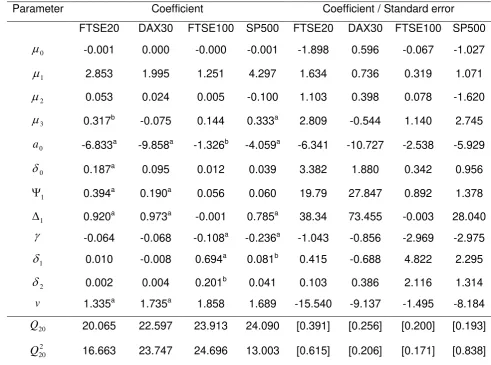
Table 1 presents the estimated parameters of model (6) for each market separately.

The standardized residuals, 1,



t A t





, and their squared values, 2,

2  t A t





, from all models obey the

standard assumptions of autocorrelation and heteroskedasticity absence. Indicatively, we present the Ljung-Box Q-statistic for the null hypothesis that there is not autocorrelation up to

20th order computed on



t



A1_,t and 2 , 2  t A t





. Briefly discussing the values of the parameters, we

note that i) the relation of the conditional variance with the risk premium, although positive, is

statistically insignificant (coefficient



₁), ii) the non-synchronous trading effect is not present

in the estimated models (coefficient



₂) and iii) concerning the cases of the FTSE20 and

SP500 stock indices, the daily serial correlation is inversely related to its conditional volatility

5 _{Engle et al. (1990) evaluated the role of the information arrival process in the determination of volatility in a}

multivariate framework providing a test of two hypotheses: heat waves and meteor showers. Using meteorological analogies, they supposed that information follows a process like a heat wave so that a hot day in New York is likely to be followed by another hot day in New York but not typically by a hot day in Tokyo. On the other hand, a meteor shower in New York, which rains down on the earth as it turns, will almost surely be followed by one in Tokyo. Thus, the heat wave hypothesis is that the volatility has only country specific autocorrelation, while the meteor shower hypothesis states that volatility in one market spills over to the next. See also Kanas (1998).

6 _{For example, in the case of the FTSE20 index daily returns, the conditional variance of the DAX30 and SP500}

(coefficient



₃). Moreover, the leverage effect is not present in the Greek and German stock

markets. On the contrary, for the SP500 and FTSE100 stock indices, the estimated value of parameter



is statistically significant at 1% level of significance. The volatility spill over effect

is statistically significant for the U.K. stock market. Regarding the SP500 index daily returns, there is evidence that volatility spillovers from Frankfurt to Chicago stock market. Finally, for

the FTSE20, DAX30 and SP500 cases, parameter v is statistically different to the value of 2

at any level of significance, justifying the use of a thick-tailed distribution. The estimated value

of



₀ is about 0.187 and statistically significant only in the case of the Greek market indicating

that a non-trading day contributes less than a fifth as much to volatility as a trading day. 3 . R o l l i n g - s a m p l e d p a r a m e t e r s o f t h e a s y m m e t r i c A R C H m o d e l

Our purpose is to examine if the estimated parameters of the asymmetric ARCH model change over time and whether there is any impact of time-varying estimated parameters on

volatility forecasting accuracy. The ARCH process is estimated, at each of a sequence of points in time, using a rolling sample of constant size equal to 1000 trading days, a sample

size that is preferred7 by the majority of applied studies.

We produce one-day-ahead conditional volatility predictions for the trading days of 11th

January 2000 to 5th July 2002. Since the ARCH model is estimated at each point in time, we

use the maximum likelihood estimates at time

t



1

as starting values for the iterative

maximization algorithm at time

t

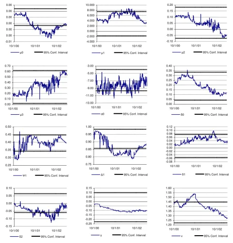
. Figure 1 depicts the rolling-sampled estimated parameters

for the FTSE20 index as well as the



2

.

06

times the conditional standard deviation

confidence interval of the parameters estimated using the full data sample8. From visual

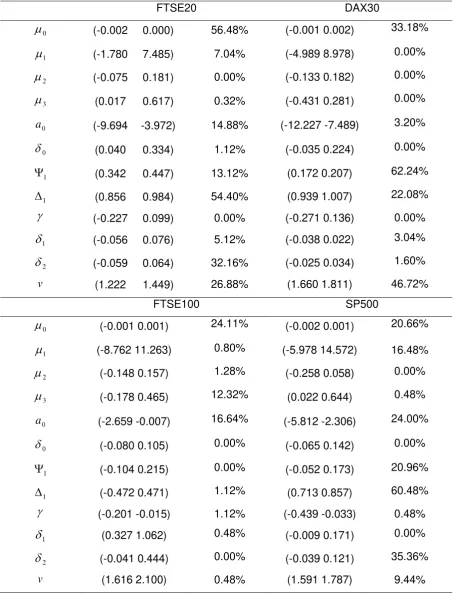
inspection, the estimated rolling parameters are, clearly, out of the confidence interval bounds in many cases. Table 2 presents the percentage of rolling-sampled estimations, which are

outside of the 95% confidence interval of the full-sampled parameters. Characteristic

examples of the change in the parameter values are



₁ and v for DAX30 as well as



₁ for

FTSE20 and SP500. However, there are rolling parameters which do not change significantly

across time, such as



(leverage effect), and



₀ (contribution of non-trading days to

volatility). An important characteristic, which is extracted from the rolling-sampled estimated

parameters, is the fact that the estimated values do not fluctuate in a mean reverting form but they change gradually. Sudden changes of the values of the rolling estimated parameters,

which are characterized by a mean reverting form, should indicate an improperly maximum likelihood estimation procedure. On the other hand, gradual changes of the estimated

7 _{Engle et al. (1993), Engle et al. (1997), Noh et al. (1994), Angelidis et al. (2004) note that the size of the rolling}

sample turns out to be rather important while Frey and Michaud (1997), Hoppe (1998) and Degiannakis and Xekalaki (2006) comment that the use of short sample sizes generates more accurate volatility forecasts, since it incorporates changes in trading behaviour more efficiently.

8 _{Figures of the estimated rolling parameters for the DAX30, FTSE100 and SP500 indices, similar to Figure 1, are}

coefficients indicate a data set that alters from time to time, forcing us to believe that the

values of the estimated parameters reflect the information that financial markets reveal. INSERT FIGURE 1 ABOUT HERE

INSERT TABLE 2 ABOUT HERE

The percentage of estimated rolling parameters that are statistically different from the parameter values estimated using the full data sample, as presented in Table 3, is also

indicative for the changes of the estimated values across time. There are four parameters, in the case of the Greek market, whose rolling-sampled estimators differ statistically significant

from their full-sampled estimators in more than 10% of the trading days. Although, in the case

of the FTSE100 index, only the rolling estimators of



₁ parameter differ statistically from their

full data sample estimator, in the case of the SP500 index there are four parameters, which

show a statistically significant difference from their full-sampled estimators in more than 20% of the trading days.

INSERT TABLE 3 ABOUT HERE

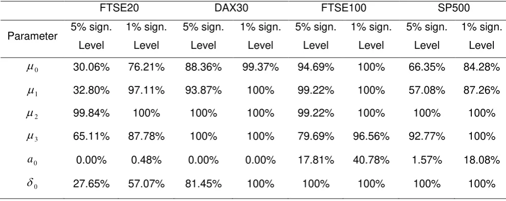
The values of the rolling parameters indicate that the characteristics of the markets change during the examined period. According to Table 4, which presents the percentage of

trading days that the rolling parameters are statistically insignificant, there are parameters

whose rolling-sampled estimations are statistically insignificant while their full-sampled

estimations are significant. For example, parameters



3 and



1 for the SP500 index, as well

as parameter



for FTSE100 index, although they appear to be significant in the full sample,

almost all their rolling-sampled estimations are insignificant at 5% level of significance. Therefore, in the full sample, an inverse relation between volatility and serial correlation

characterizes FTSE20 index, but the values of rolling



₃ are not different to zero in most of

the cases. Of course, there are parameters whose estimations are statistically different to zero

in both the full sample and the rolling samples (i.e. the parameter



₁ for the FTSE20, DAX30

and SP500 indices). Hence, we may infer that the values of the estimated parameters change across time, reflecting the individual features of particular periods that characterize financial

markets.

INSERT TABLE 4 ABOUT HERE

However, although the estimated parameters are time varying, the in-sample and out-of-sample forecasting ability of the model is accurate. There are 31, 19, 17 and 29 cases, or

4.99%, 2.99%, 2.66% and 4.57%, observed returns outside the 95% confidence intervals for the FTSE20, DAX30, FTSE100 and SP500 indices, respectively. In Figure 2.a, the 95%

in-sample confidence interval of the FTSE20 index of daily returns is plotted from 11th January

2000 to 5th July 2002. However, a model that uses a large number of parameters may exhibit

an excellent in-sample fit but a poor out-of-sample performance. Studies such as Heynen and

volatility prediction models with in-sample and out-of-sample data sets. We investigate the

possibility that model over-fitting can be occurred and evaluate the performance of the estimated ARCH model by computing the out-of-sample forecasts. In the sequel, the

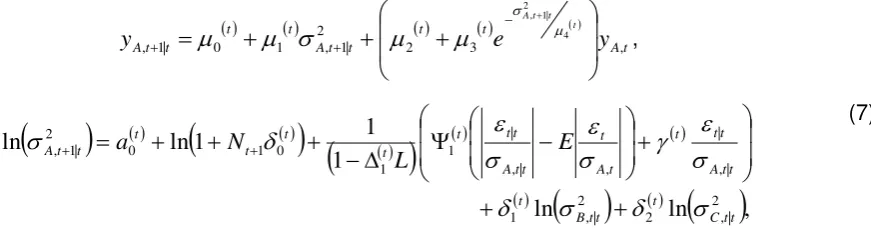
one-day-ahead 95% prediction intervals are constructed. Let us compute the one-day-one-day-ahead

conditional mean, y_t1|_t E



y_t1

 



 t |I_t



, and conditional variance,

 

 



t



t t t

t E |I

2 1 2

|

1







_  _ ,

using the following formulas:

          t A t t t t A t t t t

A

e

y

y

t t t A , 3 2 2 | 1 , 1 0 | 1 , 4 2 | 1 ,

























     











,





 



 



 





   

 _ln

 

 _ln

 

_,

1 1 1 ln ln 2 | , 2 2 | , 1 | , | , | , | 1 1 0 1 0 2 | 1 , t t C t t t B t t t A t t t t A t t t A t t t t t t t t t A E L N a



























                           _  (7)

where



 t







₀ t

,



₁ t

,



₂ t

,



₃ t

,

a

₀ t

,



₀ t

,



₁ t

,



 ₁t

,



 t

,



₁ t

,



₂ t

,

v

 t



is the parameter vector that is estimated using the sample data set which is available at time

t

,



t|t



E





t

|

I

t



denotes the prediction error conditional on the information set that is available at time

t

, and



t t



t t

A E |I

2 |

,





 is the conditional standard deviation which is computed by the ARCH

model, in equation (6), using the information set available at time

t

. Note that for



v



GED

z_t ~ 0,1; , the expected value of its absolute price is equal to

 

 



 

 

 

 



1/2

1

,

2

1

3





_

_

t

_

t

_

t

t A

t

v

v

v

[image:9.595.95.531.181.296.2]

E





.

Figure 2.b plots the one-day-ahead 95% prediction interval, which is constructed as the

one-day-ahead conditional mean



2.06 times the conditional standard deviation, both

measurable to It information set, or

 





At t t

t t

A GED v

y _,_1|  0,1; ,0.025



_,_1| , where GED



0,1;v t,a



is the

100



1



a



quantile of the GED distribution. Hence, each trading day, (

t

), the next

trading day’s, (

t



1

), prediction intervals are constructed, using only information available at

current trading day,

t

. There are 29, 22, 21 and 32 observations or 4.67%, 3.46%, 3.29% and

5.04% for the FTSE20, DAX30, FTSE100 and SP500 indices, respectively, outside the 95%

prediction intervals9.

INSERT FIGURE 2 ABOUT HERE

For a more formal method of evaluating forecasting adequacy, we apply two

hypotheses tests that measure the forecasting accuracy in a VaR framework. One-day-ahead

VaR at a given probability level, a, is the next trading day’s predicted amount of financial loss

of a portfolio, or







 



At t

t

t a GED v a

VaR_1|11  0,1; ,



_,_1| . Kupiec (1995) introduced a likelihood

9 _{Figures, similar to Figure 2, that depict the in-sample 95% confidence interval and the one-day-ahead 95%}

ratio statistic for testing the null hypothesis that the proportion of confidence interval violations

is not larger than the VaR forecast. The test statistic, which is asymptotically X12 distributed,

is computed as 2[ln(( )n(1 )N n) ln( n(1 )N n]

K n N n N p p

LR       , where



n



_iN_1d



yt_1VaRt_1|t



a/2







d



y

t1



VaR

t1|t



1



a

/

2





is the number of trading days over

the out-of-sample period

N

that a violation has occurred, for

d



y

_t1



VaR

_t1|t

 

a

/

2





1

if

t t t

VaR

y

_1



_1| and

d



y

t₁



VaR

t_1|t

 

a

/

2





0

otherwise, and p is the expected frequency of violations. Christoffersen (1998) developed a likelihood ratio statistic that jointly investigates

whether i) the proportion of violations is not larger than the VaR forecast and ii) the violations

are independently distributed. The statistic is computed as LRC -2ln((1 ) )

n n N

p p 



)) )

1 ( )

1 (

2ln( 00 01 10 11

11 11 01

01

n n n

n













 , where 



j ij ij ij n n



and

n

_ij is the number of

observations with value i followed by j, for

i

,

j



0

,

1

. The values

i

,

j



1

denote that a

violation has been made, while

i

,

j



0

indicate the opposite. Under the null hypothesis, the

C

LR is asymptotically chi-squared distributed with two degrees of freedom. The main

advantage of Christoffersen’s test is that it can reject a VaR model that generates either too

many or too few clustered violations. Both tests do not reject the null hypothesis of correct

proportion of violations in all the cases, except for the 95%-VaR of the FTSE100 index. In the

case of Kupiec’s test the p-values are 70.28%, 6.08%, 3.45% and 96.37% for 95%-VaR and

8,15%, 13.63%, 56.56% and 52.70% for 99%-VaR, for the FTSE20, DAX30, FTSE100 and SP500 indices, respectively. Testing the null hypothesis of whether the violations are equal to

the expected ones as well as if they are independent, we observe that the relative p-values are 40.03%, 16.42%, 0.15% and 95.19% in the 95%-VaR case and 17.98%, 32.51%, 7.10%

and 73.92% in the 99%-VaR case, for the FTSE20, DAX30, FTSE100 and SP500 indices, respectively.

Despite the fact that the values of the estimated coefficients change over time, the model adequately forecasts the one-day-ahead volatility. Thus, changes in the values of the estimated parameters do not indicate inadequacy of the model in describing the data. On the

contrary, model’s parameters should be re-estimated on a daily base in order to reflect any changes that have been occurred in the stock market and have been incorporated in the

prices of assets10.

10

4 . R o l l i n g - s a m p l e d p a r a m e t e r s f r o m s i m u l a t e d p r o c e s s e s

A simulation study could shed light in rolling-sampled estimated parameters’ behaviour. A series of simulations is run in order to investigate if the time-variant attitude holds even in the

case of an ARCH data generating process. We generate a series of 32000 values from the

standard normal distribution, ~

 

0,1

. . .

N z

d i i

t . Then an AR(1)GARCH(1,1) process is created,

 

32000 1



t t

y , where yt 0.00050.15yt1



t, by multiplying the i.i.d. process with a specific

conditional variance form



t zt



t2 , for

2 1 2

1 2

90

.

0

05

.

0

0005

.

0











_{t t}

t







. The

AR(1)GARCH(1,1) model is applied on the

 

yt 32000_t1002 generated data. Dropping out the first

1001 data, maximum likelihood rolling-sampled estimates of the parameters are obtained by numerical maximization of the log-likelihood function, using a rolling sample of constant size

equal to 1000. According to Table 5, about 58% of the 30000 conditional variance rolling-sampled parameters are outside the 95% confidence interval of the parameters estimated

using the whole sample set of the 30000 simulated data. The procedure is repeated for an

AR(1)EGARCH(1,1) conditional variance form,

 

₁

 

2₁

1 1

1 1 1 0 2

ln

ln 

  

 _{ }



 _t

t t t

t

t a a

_















,

but the results are robust to the choice of the conditional variance specification.

A series of 32000 values from the first order autoregressive process are also

produced. The AR(1) process is created as y_t 0.00010.12y_t1z_t, for ~

 

0,1

. . .

N z

d i i

t .

Dropping out the first 1001 data, 30000 maximum likelihood rolling-sampled estimates of the

parameters are also obtained. As far as the case of the AR(1) process is concerned, we infer that the rolling estimated parameters are time-invariant, as on average 5% of the estimated

rolling parameters are outside the 95% confidence levels.

Both the AR(1)GARCH(1,1) and the AR(1) processes were simulated for various sets

of parameters, but there are no qualitative differences to the fore mentioned conclusions. Moreover, a series of simulations were repeated i) for ARCH volatility forms without any

conditional mean specification, ii) based on estimation procedures of the most well known

packages, EVIEWS® 4.1 and OX-G@ARCH® 3.4, iii) for larger rolling samples of 5000 values,

iv) for non-overlapping data samples, but there were no qualitative differences in any of these cases11.

So, the simulation study provides evidence that the time-variant attitude of rolling-sampled parameters estimations characterizes not only the examined data sets but the ARCH

data generating process itself as well.

INSERT TABLE 5 ABOUT HERE

likelihood algorithm at time t. Despite the slight changes occurred in each case, the rolling parameters are time-variant for all cases.

5 . R o l l i n g - s a m p l e d p a r a m e t e r s f r o m a L e v y - s t a b l e d i s t r i b u t i o n In this section, we investigate whether the phenomenon of parameter changing across time is related with the unconditional distribution of returns also. Mandelbrot (1963) and Fama (1965)

made the first re-examination of the unconditional distribution of stock returns. Mandelbrot (1963) concluded that price changes can be characterized by a stable Paretian distribution with a characteristic exponent, a, less than two, thus exhibiting fat tails and infinite variance.

Fama (1965) examined the distribution of thirty stocks of the Dow Jones Industrial Average;

his results were consistent with Mandelbrot’s. Thereafter, it has been accepted that the stock

returns distributions are fat-tailed and peaked. In an attempt to model the unconditional distribution of stock returns several researchers have considered alternative approaches. See

for example, Blattberg and Gonedes (1974), Bradley and Taqqu (2002), Clark (1973), Kon (1984), McDonald (1996), Mittnik and Rachev (1993), Panas (2001), Rachev and Mittnik

(2000).12

The probability density function of a stable distribution cannot be described in a closed

mathematical form. By definition, a univariate distribution function is stable if and only if its characteristic function has the form

 

 























































t

a

t

t

i

t

t

i

t

exp





a

1





,



,

8)

where

i





1

,

t



R

,

 



     

2 tan

,





t a if

a



1

and

 

t

,

a

2

log

t









if

a



1

. The

particular distribution represented by its characteristic function is determined by the values of

four parameters: a,



,



and



. The parameter a,

0







2

, is called the characteristic

exponent. It measures the thickness of the tails of a stable distribution. The smaller the value

a, the higher the probability in the distribution tails. If

a



2

then we have thicker tails than the

tails of normal distribution. Thus, stable distributions have thick tails and consequently

increase the likelihood of the occurrence of large shocks. The skewness parameter



,

1

1









, is a measure of the asymmetry of the distribution. The distribution is symmetric, if

0





. As



approaches one, the degree of skewness increases. The scale parameter



,

0





, is a measure of the spread of the distribution. It is similar to the variance of the normal

distribution,







2

. However, the scale parameter



is finite for all stable distributions,

despite the fact that the variance is infinite for all

a



2

. The location parameter



,













, is the mean of the distribution, for

a



1

, and the median for

0



a



1

. The

12 _{De Vries (1991), Ghose and Kroner (1995) and Groenendijk et al. (1995) demonstrate that ARCH models share}

case of

a



2

,





0

corresponds to the normal distribution, while

a



1

,





0

corresponds

to the Cauchy distribution.

In estimating the parameters of the stable distribution of index returns, we adopt the

estimation procedure suggested by McCulloch (1986). The estimation procedure is a quantile

method and works for

0

.

6



a



2

and any value of the other parameters. Essentially,

McCulloch suggests that if we have a random variable x, which follows a stable distribution

and denotes the pth quantile of this distribution by

x

 

p

, then the population quantile can be estimated by the sample quantile

x

ˆ

 

p

. McCulloch’s estimator uses five quantiles to estimate

a and



as

  

 





0

.

75

 

ˆ

0

.

25



ˆ

05

.

0

ˆ

95

.

0

ˆ

ˆ

x

x

x

x











and

  

 









0

.

95

 

ˆ

0

.

05



ˆ

50

.

0

ˆ

2

05

.

0

ˆ

95

.

0

ˆ

ˆ

x

x

x

x

x













. Since



 

a

is

monotonic in a and



 



is monotonic in



, we are able to find a and



by inverting



 

a

and



 



, thus

a

ˆ



g

₁





ˆ

   

a

,



ˆ





and



ˆ



g

₂





ˆ

   

a

,



ˆ





. McCulloch tabulated

g

₁ and

g

₂ for

various values of



 

a

and



 



. A similar procedure is also applied for the scale and location

parameters. An alternative procedure to estimate the parameters of the stable distribution is

the regression method proposed by Koutrouvelis (1980).

Following a procedure similar to that of ARCH modelling, the parameters of the stable

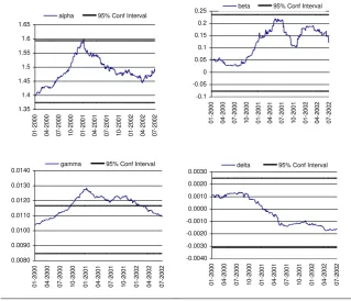
distribution are estimated, at each of a sequence of points in time, using a rolling sample of constant size equal to 1000 trading days. The empirical findings, for the case of the Greek

stock market, are graphically summarized in Figure 3, which plots the rolling-sampled estimates of parameters along with the 95% confidence interval of the parameters estimated

using the full data sample. Inspection of Figure 3 shows that the estimates of a are less than

two. The case of FTSE20 reveals that 92% of the a’s rolling-sampled estimates are between

1.44 and 1.55. The parameter



is greater than zero, which implies skewness to the right.

The rolling values of



are positive and range from 0.003 to 0.22 but there are not outside the

95% confidence interval for any case13.

INSERT FIGURE 3 ABOUT HERE

In Table 6, we present the estimates of the parameters of stable distribution based on all data available as well as the standard deviation of the rolling-sampled estimated parameters. The estimates of a do not approach the value of two in any of the examined

indices. However, there are estimated rolling parameters that are statistically different from the parameter values estimated using the full data sample. For example, the rolling-sampled

estimates of the tail index (a) are statistically different to the full sample estimated parameter

in the 51.46% of the trading days for the case of the SP500 index. The rolling estimates of

13 _{Figures depicting the rolling-sampled estimates of the parameters for the DAX30, FTSE100 and SP500 indices}

parameter



are statistically different to the relevant full-sampled values in 9.59% and 9.42%

of the trading days for the DAX30 and FTSE100 indices, respectively, whereas the location ( ) parameters are time-variant in none of the cases. Another important parameter of the stable distribution, from the point of view of portfolio theory, is the scale parameter,



. As far

as the FTSE20 index is concerned, the rolling-sampled estimates of the scale parameter differ statistically from its full-sampled value in the 56.48% of the trading days. Hence, the

parameter estimates, using the full data sample are statistically different from the parameter values estimated using the rolling samples of constant size for one parameter in each index.

INSERT TABLE 6 ABOUT HERE 6 . D i s c u s s i o n

We estimated an asymmetric ARCH model using daily returns of the FTSE20, DAX30, FTSE100 and SP500 indices and concluded that although the estimated parameters of the

model change over time, the model does not lose its ability to forecast the one-day-ahead volatility accurately. Furthermore, the rolling parameter analysis was applied to the

unconditional distribution of returns. We observed the phenomenon of parameter changing across time for both the conditional (ARCH process) and the unconditional (Levy-stable) distribution of returns. Even in the case of a simulated ARCH process, the property of time

varying rolling-sampled parameters holds. One possible reason for parameter instability might

be that the behaviour of the market participants has undergone fundamental changes. Parameters instability indicates a change in market behavior but we can not determine the source of that change. The term ‘a data set that alters’, could incorporate a wide range of

possible sources, i.e. financial legislation, market microstructure, market participants’

perspective, technological revolution or even macroeconomic policy.

Gallant et al. (1991), Stock (1988), Lamoureux and Lastrapes (1990) and Schwert (1989) among others have aimed at explaining the economic interpretation of the ARCH

process. As Engle et al. (1990) and Lamoureux and Lastrapes (1990) have noted, the explanation of the ARCH process must lie either in the arrival process of news or in market

dynamics in response to the news. Based on some earlier work by Clark (1973) and Tauchen and Pitts (1983), Gallant et al. (1991) provided a theoretical interpretation of the ARCH effect.

They assumed that the asset returns are defined by a stochastic number of intra-period price revisions and information flows into the market in an unknown rate. As the daily information does not come to the stock market in a constant and known rate, the estimation of the ARCH

stochastic process that explains the dynamics of the stock market could be revised at regular time intervals. In our case the ARCH process is estimated using daily returns. Thus, the

parameters of the model may be revised on a daily base, because of the observed phenomenon of changes in the estimated parameters. If we used data of higher frequency, i.e.

To the best of authors’ knowledge, this is the first study that investigates the

phenomenon of time varying estimated parameters either i) in real-world financial data or ii) in a simulated data generating process. A natural extension of this study would be to analyse the

change and the relative economic interpretation of the estimated values of the parameters in intra-daily high-frequency data sets.

A c k n o w l e d g e m e n t

We would like to thank the editor and an anonymous referee for their constructive comments that helped to improve significantly an earlier version of the paper.

R e f e r e n c e s

Andersen, T. and Bollerslev, T. (1998). ARCH and GARCH Models, Encyclopedia of

Statistical Sciences Vol.II, (eds.) Samuel Kotz, Campbell B. Read and David L. Banks, New York, John Wiley and Sons Inc.

Angelidis, T., Benos, A. and Degiannakis, S. (2004). The Use of GARCH Models in VaR Estimation. Statistical Methodology, 1(2), 105-128.

Balaban, E. and Bayar, A. (2005). Stock returns and volatility: empirical evidence from fourteen countries. Applied Economics Letters, 12, 603-611.

Barndorff-Nielsen, O.E., Nicolato, E. and Shephard, N. (2002). Some Recent Developments in

Stochastic Volatility Modelling. Quantitative Finance, 2, 11-23.

Bera, A.K. and Higgins, M.L. (1993). ARCH Models: Properties, Estimation and Testing. Journal of Economic Surveys, 7, 305-366.

Berndt, E., Hall, B., Hall, R. and Hausman, J. (1974). Estimation and Inference in Nonlinear

Structural Models. Annals of Economic and Social Measurement, 3, 653-665.

Black, F. (1976). Studies of Stock Market Volatility Changes. Proceedings of the American Statistical Association, Business and Economic Statistics Section, 177-181.

Blattberg, R.C. and Gonedes, N.J. (1974). A comparison of the stable and student distributions as statistical models for stock prices. Journal of Business, 47, 244-80.

Blair, B.J., Poon, S.-H. and Taylor, S.J. (2001). Forecasting S&P 100 volatility: the incremental

information content of implied volatilities and high frequency index returns. Journal of Econometrics, 105, 5-26.

Bollerslev, T., Chou, R. and Kroner, K.F. (1992). ARCH Modeling in Finance: A Review of the

Theory and Empirical Evidence. Journal of Econometrics, 52, 5-59.

Bollerslev, T., Engle, R.F. and Nelson, D. (1994). ARCH Models. In: R.F. Engle and D.

McFadden (Eds.), Handbook of Econometrics, Volume 4, Elsevier Science, Amsterdam,

2959-3038.

Bradley, B. and Taqqu, M. (2002). Financial Risk and Heavy Tails. In: S. Rachev (Ed.),

Heavy-tailed distributions in Finance, North-Holland.

Campbell, J., Lo, A. and MacKinlay, A.C. (1997). The Econometrics of Financial Markets. New Jersey. Princeton University Press.

Chib, S., Kim, S. and Shephard, N. (1998). Stochastic Volatility: Likelihood Inference and

Comparison with ARCH Models. Review of Economic Studies, 65, 361-393.

Christoffersen, P. (1998). Evaluating interval forecasts. International Economic Review, 39, 841-62.

Clark, P.K. (1973). A Subordinated Stochastic Process Model with Finite Variance for Speculative Prices. Econometrica, 41, 135-156.

Degiannakis, S. (2004). Volatility Forecasting: Evidence from a Fractional Integrated

Asymmetric Power ARCH Skewed-t Model. Applied Financial Economics, 14, 1333-1342.

Degiannakis, S. and Xekalaki, E. (2001). Using a Prediction Error Criterion for Model Selection in Forecasting Option Prices. Athens University of Economics and Business, Department of

Statistics, Technical Report, 131. Available online at:

http://stat-athens.aueb.gr/~exek/papers/Xekalaki-TechnRep131(2001a)ft.pdf.

Degiannakis, S. and Xekalaki, E. (2004). Autoregressive Conditional Heteroscedasticity

Models: A Review. Quality Technology and Quantitative Management, 1(2), 271-324.

Degiannakis, S. and Xekalaki, E. (2006). Assessing the Performance of a Prediction Error

Criterion Model Selection Algorithm in the Context of ARCH Models, Applied Financial

Economics, forthcoming.

De Vries, C.G. (1991). On the Relation Between GARCH and Stable Processes. Journal of Econometrics, 48, 313-324.

Diebold, F.X. (2003). The ET Interview: Professor Robert F. Engle. Econometric Theory, 19,

1159-1193.

Ding, Z., Granger, C.W.J. and Engle, R.F. (1993). A Long Memory Property of Stock Market

Returns and a New Model. Journal of Empirical Finance, 1, 83-106.

Engle, R.F., Lilien, D.M. and Robins, R.P. (1987). Estimating Time Varying Risk Premia in the

Term Structure: The ARCH-M Model. Econometrica, 55, 391–407.

Engle, R.F., Ito, T. and Lin, W.L. (1990). Meteor Showers or Heat Waves? Heteroskedastic Intra-Daily Volatility in the Foreign Exchange Market. Econometrica, 58, 525-542.

Engle, R.F., Hong, C., Kane, A. and Noh, J. (1993). Arbitrage Valuation of Variance Forecasts

with Simulated Options, Advances in Futures and Options Research, 6, 393-415.

Engle, R.F., Kane, A. and Noh, J. (1997). Index-Option Pricing with Stochastic Volatility and

the Value of Accurate Variance Forecasts. Review of Derivatives Research, 1, 120-144.

Fama, E.F. (1965). The Behaviour of Stock Market Prices. Journal of Business, 38, 34-105.

French, K.R. and Roll, R. (1986). Stock Return Variances: The Arrival of Information and the Reaction of Traders. Journal of Financial Economics, 17, 5-26.

Gallant, A.R., Hsieh, D.A. and Tauchen, G. (1991). On Fitting a Recalcitrant Series: The

Pound/Dollar Exchange Rate 1974-83. In: W.A. Barnett, J. Powell, and G. Tauchen (Eds.), Nonparametric and Semiparametric Methods in Econometrics and Statistics, Cambridge University Press, Cambridge.

Ghose, D. and Kroner, K.F. (1995). The relationship between GARCH and symmetric stable processes: Finding the source of fat tails in financial data. Journal of Empirical Finance, 2, 225–251.

Groenendijk, P.A., Lucas, A. and de Vries, C.G. (1995). A note on the relationship between

GARCH and symmetric stable processes. Journal of Empirical Finance, 2, 253–264.

Ghysels, E., Harvey, A. and Renault, E. (1996). Stochastic Volatility. In: G.S. Maddala (Ed.),

Handbook of Statistics, Vol. 14, Statistical Methods in Finance, 119-191, Amsterdam, North Holland.

Giot, P. and Laurent, S. (2003). Value-at-Risk for Long and Short Trading Positions. Journal of

Applied Econometrics, 18, 641-664.

Heynen, R. and Kat, H. (1994). Volatility Prediction: A Comparison of the Stochastic Volatility,

GARCH(1,1), and EGARCH(1,1) Models, Journal of Derivatives, Winter, 94, 50-65.

Hol, E. and Koopman, S. (2000). Forecasting the Variability of Stock Index Returns with

Stochastic Volatility Models and Implied Volatility, Tinbergen Institute, Discussion Paper No.

104, 4.

Hoppe, R. (1998). VAR and the Unreal World, Risk, 11, 45-50.

Jacquier, E., Polson, N. and Rossi, P. (1999). Stochastic Volatility: Univariate and Multivariate

Extensions. CIRANO, Scientific Series, 99s, 26.

Kanas, A. (1998). Volatility Spillovers Across Equity Markets: European Evidence. Applied Financial Economics, 8, 245-256.

Kupiec, P.H. (1995). Techniques for verifying the accuracy of risk measurement models, Journal of Derivatives, 3, 73-84.

Kon, S.J. (1984). Models of stock returns – A comparison. Journal of Business, 39, 147-165. Koutrouvelis, I.A. (1980). Regression-Type Estimation of the Parameter of Stable Laws.

Journal of the American Statistical Association, 75, 918-928.

Lamoureux, G.C. and Lastrapes, W.D. (1990). Heteroskedasticity in Stock Return Data:

Volume Versus GARCH Effects. Journal of Finance, 45, 221-229.

LeBaron, B. (1992). Some Relations Between Volatility and Serial Correlations in Stock

Market Returns. Journal of Business, 65, 199-219.

Liu, S.M. and Brorsen, B.W. (1995). Maximum likelihood estimation of a GARCH-stable

model. Journal of Applied Econometrics, 10, 273–285.

Marquardt, D.W. (1963). An Algorithm for Least Squares Estimation of Nonlinear Parameters. Journal of the Society for Industrial and Applied Mathematics, 11, 431-441.

McCulloch, J.H. (1986). Simple Consistent Estimates of Stable Distribution Parameters. Communications in Statistics: Simulation and Computation, 15, 1109-1136.

McDonald, J.B. (1996). Probability Distributions for Financial Models. In: G.S. Maddala and C.R. Rao (Eds.), Statistical Methods in Finance, vol. 14, Handbook of Statistics, Elsevier, Amsterdam.

Mittnik, S. and Rachev, S.T. (1993). Modelling Asset Returns with Alternative Stable

Distributions, Economic Review, 12, 261-330.

Mittnik, S., Rachev, S.T., Doganoglu, T. and Chenyao, D. (1999). Maximum Likelihood

Estimation of Stable Paretian Models. Mathematical and Computer Modelling, 29, 275-293.

Nelson, D. (1991). Conditional Heteroskedasticity in Asset Returns: A New Approach.

Econometrica, 59, 347-370.

Noh, K., Engle, R.F. and Kane, A. (1994). Forecasting Volatility and Option Prices of the S&P 500 Index. Journal of Derivatives, 2, 17-30.

Pagan, A. and Schwert, G. (1990). Alternative Models for Conditional Stock Volatility, Journal

of Econometrics, 45, 267-290.

Panas, E. (2001). Estimating Fractal Dimension Using Stable Distributions and Exploring Long

Memory Through ARFIMA Models in Athens Stock Exchange. Applied Financial

Economics, 11, 395-402.

Panorska, A., Mittnik, S. and Rachev, S.T. (1995). Stable GARCH Models for Financial Time

Series. Applied Mathematics Letters, 8, 33-37.

Poon, S.H. and Granger, C.W.J. (2003). Forecasting Volatility in Financial Markets: A Review.

Journal of Economic Literature, XLI, 478-539.

Rachev, S. and Mittnik, S. (2000). Stable Paretian Models in Finance, John Wiley.

Schwert, G.W. (1989). Why Does Stock Market Volatility Changes Over Time. Journal of

Finance, 44, 1115-1153.

Shephard, N. (2004). Stochastic Volatility: Selected Readings, Oxford University Press.

Stock, J.H. (1988). Estimating Continuous Time Process Subject to Time Deformation. Journal

of the American Statistical Association, 83, 77-85.

Tauchen, G. and Pitts, M. (1983). The Price Variability-Volume Relationship on Speculative Markets. Econometrica, 51, 485-505.

Taylor, S.J. (1994). Modelling Stochastic Volatility. Mathematical Finance, 4(2), 183-204. Tsionas, E.G. (2002). Likelihood-Based Comparison of Stable Paretian and Competing

Models: Evidence from Daily Exchange Rates. Journal of Statistical Computation and

Simulation, 72(4), 341-353.

[image:20.595.65.557.132.497.2]

T a b l e s a n d F i g u r e s

Table 1. Parameter estimates for the FTSE20, DAX30, FTSE100 and SP500 index daily returns

(January 3rd, 1996 to July 5th, 2002).

Parameter Coefficient Coefficient / Standard error

FTSE20 DAX30 FTSE100 SP500 FTSE20 DAX30 FTSE100 SP500

0



-0.001 0.000 -0.000 -0.001 -1.898 0.596 -0.067 -1.027

1



2.853 1.995 1.251 4.297 1.634 0.736 0.319 1.071

2



0.053 0.024 0.005 -0.100 1.103 0.398 0.078 -1.620

3



0.317b -0.075 0.144 0.333a 2.809 -0.544 1.140 2.745

0

a -6.833a -9.858a -1.326b -4.059a -6.341 -10.727 -2.538 -5.929

0



0.187a 0.095 0.012 0.039 3.382 1.880 0.342 0.956

1



0.394a 0.190a 0.056 0.060 19.79 27.847 0.892 1.378

1



0.920a 0.973a -0.001 0.785a 38.34 73.455 -0.003 28.040



_{-0.064 -0.068 -0.108}a

-0.236a -1.043 -0.856 -2.969 -2.975

1



0.010 -0.008 0.694a 0.081b 0.415 -0.688 4.822 2.295

2



0.002 0.004 0.201b 0.041 0.103 0.386 2.116 1.314

v 1.335a 1.735a 1.858 1.689 -15.540 -9.137 -1.495 -8.184

20

Q 20.065 22.597 23.913 24.090 [0.391] [0.256] [0.200] [0.193]

2 20

Q

16.663 23.747 24.696 13.003 [0.615] [0.206] [0.171] [0.838]

Notes: With v=1.335, v=1.735, v=1.858, v=1.689, the 97.5% point of the generalized error distribution

are 2.06, 2.00, 1.98 and 2.00, respectively. With v=1.335, v=1.735, v=1.858, v=1.689, the 99.5% point

of the generalized error distribution are 2.94, 2.70, 2.65 and 2.72, respectively. For the FTSE20 index,

parameters



₁ and



₂ present the volatility spillover from the SP500 and DAX30 indices, respectively. For

the DAX30 index, parameters



₁ and



₂ present the volatility spillover from the FTSE100 and SP500

indices, respectively. For the FTSE100 index, parameters



₁ and



₂ present the volatility spillover from

the DAX30 and SP500 indices, respectively. For the SP500 index, parameters



₁ and



₂ present the

volatility spillover from the DAX30 and FTSE100 indices, respectively. Q₂₀ and

Q

₂₀2 are the Q-statistics of

order 20 computed on the standardized residuals and their squared values, respectively. The relative

p-values are presented in brackets.

a

Indicates that the coefficient is statistically significant at 1% level of significance.

b

Table 2. Percentage of rolling-sampled estimated parameters that are outside the 95% confidence interval. (Values in parenthesis present the lower and upper bounds of the 95%

confidence interval).

FTSE20 DAX30

0



(-0.002 0.000) 56.48% (-0.001 0.002) 33.18%

1



(-1.780 7.485) 7.04% (-4.989 8.978) 0.00%

2



(-0.075 0.181) 0.00% (-0.133 0.182) 0.00%

3



(0.017 0.617) 0.32% (-0.431 0.281) 0.00%

0

a (-9.694 -3.972) 14.88% (-12.227 -7.489) 3.20%

0



(0.040 0.334) 1.12% (-0.035 0.224) 0.00%

1



(0.342 0.447) 13.12% (0.172 0.207) 62.24%

1



(0.856 0.984) 54.40% (0.939 1.007) 22.08%



_{(-0.227 0.099) 0.00% (-0.271 0.136)} 0.00%

1



(-0.056 0.076) 5.12% (-0.038 0.022) 3.04%

2



(-0.059 0.064) 32.16% (-0.025 0.034) 1.60%

v (1.222 1.449) 26.88% (1.660 1.811) 46.72%

FTSE100 SP500

0



(-0.001 0.001) 24.11% (-0.002 0.001) 20.66%

1



(-8.762 11.263) 0.80% (-5.978 14.572) 16.48%

2



(-0.148 0.157) 1.28% (-0.258 0.058) 0.00%

3



(-0.178 0.465) 12.32% (0.022 0.644) 0.48%

0

a (-2.659 -0.007) 16.64% (-5.812 -2.306) 24.00%

0



(-0.080 0.105) 0.00% (-0.065 0.142) 0.00%

1



(-0.104 0.215) 0.00% (-0.052 0.173) 20.96%

1



(-0.472 0.471) 1.12% (0.713 0.857) 60.48%



_{(-0.201 -0.015) 1.12% (-0.439 -0.033) 0.48%}

1



(0.327 1.062) 0.48% (-0.009 0.171) 0.00%

2



(-0.041 0.444) 0.00% (-0.039 0.121) 35.36%

[image:21.595.88.546.134.728.2]

[image:22.595.84.547.115.471.2]

Table 3. Percentage of rolling-sampled estimated parameters that are statistically different from the parameter values estimated using the full data sample.

FTSE20 DAX30 FTSE100 SP500

Parameter

5% sign.

Level

1% sign.

Level

5% sign.

Level

1% sign.

Level

5% sign.

Level

1% sign.

Level

5% sign.

Level

1% sign.

Level

0



21.86% 1.29% _{13.67% 0.80% 4.02% 0.00% 14.15% 4.34%}

1



0.96% 0.00% _{0.00% 0.00% 0.16% 0.00% 8.52% 0.64%}

2



0.00% 0.00% _{0.00% 0.00% 1.13% 0.00% 0.00% 0.00%}

3



0.00% 0.00% _{0.00% 0.00% 3.22% 0.64% 0.00% 0.00%}

0

a 17.20% 3.86% _{16.72% 7.40% 0.48% 0.00% 24.28% 6.59%}

0



0.00% 0.00% _{0.00% 0.00% 0.00% 0.00% 2.73% 0.00%}

1



7.40% 0.00% _{0.00% 0.00% 0.00% 0.00% 7.56% 0.00%}

1



18.97% 10.13% _{2.57% 0.00% 14.47% 5.79% 31.67% 3.54%}



_{0.00% 0.00% 5.14% 0.00% 4.50% 0.00% 36.17% 10.13%}

1



0.00% 0.00% _{0.00% 0.00% 0.80% 0.32% 0.00% 0.00%}

2



12.54% 0.16% _{0.00% 0.00% 0.16% 0.00% 24.92% 0.00%}

v 1.29% 0.00% 16.72% 0.32% 0.00% 0.00% 0.00% 0.00%

Table 4. Percentage of the rolling-sampled estimated parameters that are statistically insignificant at 5% and 1% levels of significance.

FTSE20 DAX30 FTSE100 SP500

Parameter 5% sign.

Level

1% sign. Level

5% sign. Level

1% sign. Level

5% sign. Level

1% sign. Level

5% sign. Level

1% sign. Level

0



30.06% 76.21% 88.36% 99.37% 94.69% 100% 66.35% 84.28%

1



32.80% 97.11% 93.87% 100% 99.22% 100% 57.08% 87.26%

2



99.84% 100% 100% 100% 99.22% 100% 100% 100%

3



65.11% 87.78% 100% 100% 79.69% 96.56% 92.77% 100%

0

a 0.00% 0.48% 0.00% 0.00% 17.81% 40.78% 1.57% 18.08%

0

[image:22.595.54.572.569.775.2]