Dynamical model for the quantum-to-classical crossover of shot noise
J. Tworzydło,1,2A. Tajic,1H. Schomerus,3and C. W. J. Beenakker1 1
Instituut-Lorentz, Universiteit Leiden, P.O. Box 9506, 2300 RA Leiden, The Netherlands 2Institute of Theoretical Physics, Warsaw University, Hoz˙a 69, 00–681 Warsaw, Poland
3Max Planck Institute for the Physics of Complex Systems, No¨thnitzer Strasse 38, 01187 Dresden, Germany 共Received 15 April 2003; published 25 September 2003兲
We use the open kicked rotator to model the chaotic scattering in a ballistic quantum dot coupled by two point contacts to electron reservoirs. By calculating the system-size-over-wave-length dependence of the shot-noise power we study the crossover from wave to particle dynamics. Both a fully quantum-mechanical and a semiclassical calculation are presented. We find numerically in both approaches that the noise power is reduced exponentially with the ratio of Ehrenfest time and dwell time, in agreement with analytical predictions.
DOI: 10.1103/PhysRevB.68.115313 PACS number共s兲: 73.23.⫺b, 05.45.Mt, 03.65.Sq, 72.70.⫹m
I. INTRODUCTION
Noise plays a uniquely informative role in connection with the particle-wave duality.1This has been appreciated for light since Einstein’s theory of photon noise. Recent theoretical2– 6and experimental7 works have used electronic shot noise in quantum dots to explore the crossover from particle to wave dynamics. Particle dynamics is deterministic and noiseless, while wave dynamics is stochastic and noisy.8 The crossover is governed by the ratio of two time scales, one classical and one quantum. The classical time is the mean dwell timeDof the electron in the quantum dot. The quantum time is the Ehrenfest time E, which is the time it takes a wave packet of minimal size to spread over the entire system. WhileDis independent ofប, the timeE increases ⬀ln(1/ប) for chaotic dynamics. An exponential suppression ⬀exp(⫺E/D) of the shot-noise power in the classical limit ប→0 共or equivalently, in the limit system-size-over-wave-length to infinity兲 was predicted by Agam, Aleiner, and Larkin.2 A recent experiment by Oberholzer, Sukhorukov, and Scho¨nenberger7fits this exponential function. However, the accuracy and range of the experimental data is not suffi-cient to distinguish this prediction from competing theories 共notably the rational function predicted by Sukhorukov9 for short-range impurity scattering兲.
Computer simulations would be an obvious way to test the theory in a controlled model 共where one can be certain that there is no weak impurity scattering to complicate the interpretation兲. However, the exceedingly slow共logarithmic兲 growth ofE with the ratio of system size over wave length has so far prevented a numerical test. Motivated by a recent successful computer simulation of the Ehrenfest-time depen-dent excitation gap in the superconducting proximity effect,10we use the same model of the open kicked rotator to search for the Ehrenfest-time dependence of the shot noise.
The reasoning behind this model is as follows. The physi-cal system we seek to describe is a ballistic共clean兲quantum dot in a two-dimensional electron gas, connected by two bal-listic leads to electron reservoirs. While the phase space of this system is four dimensional, it can be reduced to two dimensions on a Poincare´ surface of section.11,12 The open kicked rotator10,13–15 is a stroboscopic model with a two-dimensional phase space that is computationally more
trac-table, yet has the same phenomenology as open ballistic quantum dots.
We study the model in two complementary ways. First we present a fully numerical, quantum-mechanical solution. Then we compare with a partially analytical, semiclassical solution, which is an implementation for this particular model of a general scheme presented recently by Silvestrov, Goorden, and one of the authors.5
II. DESCRIPTION OF THE MODEL
We give a description of the open kicked rotator, both in quantum-mechanical and in classical terms.
A. Closed system
We begin with the closed system 共without the leads兲. In this section we follow Refs. 16,17. The quantum kicked ro-tator has Hamiltonian
H⫽⫺ ប
2
2I0
2
2⫹
KI0
0
cos
兺
k⫽⫺⬁⬁
␦s共t⫺k0兲. 共2.1兲
The variable 苸(0,2) is the angular coordinate of a par-ticle moving along a circle 共with moment of inertia I0), kicked periodically at time intervals 0 共with a strength ⬀K cos). To avoid a spurious breaking of time-reversal symmetry later on, when we open up the system, we repre-sent the kicking by a symmetrized delta function: ␦s(t) ⫽1
2␦(t⫺⑀)⫹ 1
2␦(t⫹⑀), with infinitesimal ⑀. The ratio ប0/2I0⬅heff represents the effective Planck constant, which governs the quantum-to-classical crossover. The stro-boscopic time0 is set to unity in most of the equations.
The stroboscopic time evolution of a wave function is given by the Floquet operatorF⫽Texp(⫺i兰00dt H/ប), where
T indicates time ordering of the exponential. For 1/heff ⬅M , an even integer, F can be represented by an M⫻M
unitary symmetric matrix. The angular coordinate and mo-mentum eigenvalues are m⫽2m/ M and Jᐉ⫽បᐉ, with
m,ᐉ⫽1,2, . . . , M . We will use rescaled variables x⫽/2 and p⫽J/បM in the range (0,1).
plays the role of the mean level spacing ␦ in the quantum dot. In coordinate representation the matrix elements of F are given by
Fmm⬘⫽共XU†⌸UX兲mm⬘, 共2.2a兲
Umm⬘⫽M⫺1/2e2imm⬘/ M, 共2.2b兲
Xmm⬘⫽␦mm⬘e⫺i( M K/4)cos(2m/ M ), 共2.2c兲 ⌸mm⬘⫽␦mm⬘e⫺im
2/ M
. 共2.2d兲
The matrix product U†⌸U can be evaluated in closed form, resulting in the manifestly symmetric expression
共U†⌸U兲mm⬘⫽M⫺1/2e⫺i/4exp关i共/ M兲共m
⬘
⫺m兲2兴. 共2.3兲Classically, the stroboscopic time evolution of the kicked rotator is described by a map on the torus 兵x, p兩modulo 1其. The map relates xk⫹1, pk⫹1 at time k⫹1 to xk, pkat time k:
xk⫹1⫽xk⫹pk⫹
K
4sin 2xk, 共2.4a兲
pk⫹1⫽pk⫹ K
4共sin 2xk⫹sin 2xk⫹1兲. 共2.4b兲
The classical mechanics becomes fully chaotic for Kⲏ7, with Lyapunov exponent ⬇ln(K/2). For smaller K the phase space is mixed, containing both regions of chaotic and of regular motion. We will restrict ourselves to the fully cha-otic regime in this paper.
For later use we give the monodromy matrix M (xk, pk), which describes the stretching by the map of an infinitesimal displacement␦xk,␦pk:
冉
␦xk⫹1␦pk⫹1
冊
⫽M共xk, pk兲
冉
␦xk
␦pk
冊
. 共2.5兲
From Eq.共2.4兲one finds
M共xk, pk兲⫽
冉
⌳共xk兲 1
⌳共xk兲⌳共xk⫹1兲⫺1 ⌳共xk⫹1兲
冊
, 共2.6a兲
⌳共x兲⫽1⫹K
2cos 2x. 共2.6b兲
B. Open system
We now turn to a description of the open kicked rotator, following Refs. 10,15,18. To model a pair of N-mode ballis-tic leads, we impose open boundary conditions in a subspace of Hilbert space represented by the indices mn(␣) in coordi-nate representation. The subscript n⫽1,2, . . . ,N labels the modes and the superscript ␣⫽1,2 labels the leads. A 2N ⫻M projection matrix P describes the coupling to the
bal-listic leads. Its elements are
Pnm⫽
再
1 if m⫽n苸兵mn(␣)其
0 otherwise. 共2.7兲
The matrices P andFtogether determine the quasienergy dependent scattering matrix
S共兲⫽P关e⫺i⫺F共1⫺PTP兲兴⫺1FPT. 共2.8兲 Using P PT⫽1, Eq.共2.8兲can be cast in the form
S⫽PAP
T⫺1
PAPT⫹1,A⫽
1⫹eiF
1⫺eiF⫽⫺A
†, 共2.9兲
which is manifestly unitary. The symmetry ofFensures that
S is also symmetric, as it should be in the presence of
time-reversal symmetry.
By grouping together the N indices belonging to the same lead, the 2N⫻2N matrix S can be decomposed into four sub-blocks containing the N⫻N transmission and reflection
matrices:
S⫽
冉
r t
t
⬘
r⬘
冊
. 共2.10兲The Fano factor F follows from19
F⫽Tr tt
†共1⫺tt†兲
Tr tt† . 共2.11兲
This concludes the description of the stroboscopic model studied in this paper. For completeness, we briefly mention how to extend the model to include a tunnel barrier in the leads.
To this end we replace Eq.共2.8兲by
S共兲⫽⫺共1⫺KKT兲1/2⫹K关e⫺i⫺F共1⫺KTK兲1/2兴⫺1FKT. 共2.12兲 The 2N⫻M coupling matrix K has elements
Knm⫽
再
冑⌫
n if m⫽n苸兵mn (␣)其0 otherwise, 共2.13兲
with⌫n苸(0,1) being the tunnel probability in mode n. Bal-listic leads correspond to ⌫n⫽1 for all n. The scattering matrix 共2.12兲 can equivalently be written in the form used conventionally in quantum chaotic scattering:20,21
S共兲⫽⫺1⫹2W共A⫺1⫹WTW兲⫺1WT, 共2.14兲 with W⫽K(1⫹
冑
1⫺KTK)⫺1 andAdefined in Eq.共2.9兲.III. QUANTUM-MECHANICAL CALCULATION
it-eration requires a multiplication by F, which can be done efficiently with the help of the fast-Fourier-transform algorithm.22,23We made sure that the iteration was fully con-verged 共error estimate 0.1%兲. In comparison with a direct matrix inversion, the iterative calculation is much quicker: the time required scales ⬀M2ln M rather than ⬀M3.
To study the quantum-to-classical crossover we reduce the quantum parameter heff⫽1/M by two orders of magnitude at fixed classical parameters D⫽M /2N⫽5,10,30 and K ⫽7,14,21.共These three values of K correspond, respectively, to Lyapunov exponents⫽1.3,1.9,2.4.兲The left edge of the leads is at m/ M⫽0.1 and m/ M⫽0.8. Ensemble averages are taken by sampling ten random values of the quasienergy 苸(0,2). We are interested in the semiclassical, large-N re-gime 共typically N⬎10). The average transmission
N⫺1
具
Tr tt†典
⬇1/2 is then insensitive to the value of heff, since quantum corrections are of order 1/N and therefore relatively small.21The Fano factor共2.11兲, however, is seen to depend strongly on heff, as shown in Fig. 1. The line through the data points follows from the semiclassical theory of Ref. 5, as explained in the following section.In Fig. 2 we have plotted the numerical data on a double-logarithmic scale, to demonstrate that the suppression of shot noise observed in the simulation is indeed governed by the Ehrenfest timeE. The functional dependence predicted for
N⬎
冑
M is5F⫽1
4e
⫺E/D,
E⫽⫺1ln共N2/ M兲⫹c, 共3.1兲
with c being a K-dependent coefficient of order unity. As shown in Fig. 2, the data follows quite nicely the logarithmic scaling with N2/ M⫽M /(2
D)2 predicted by Eq.共3.1兲. This corresponds to a scaling with w2/LF in a two-dimensional quantum dot 共with F being the Fermi wave length and w and L the width of the point contacts and of the dot, respec-tively兲. We note that the same parametric scaling governs the quantum-to-classical crossover in the superconducting prox-imity effect.10,24
IV. SEMICLASSICAL CALCULATION
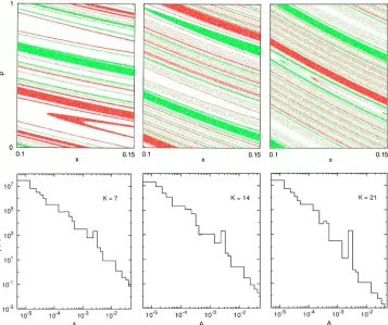
To describe the data from our quantum-mechanical simu-lation we use the semiclassical approach of Ref. 5. To that end we first identify which points in the x, p phase space of lead 1 are transmitted to lead 2 and which are reflected back to lead 1. By iteration of the classical map共2.4兲we arrive at phase-space portraits as shown in Fig. 3 共top panels兲. Points of different color 共or gray scale兲 identify the initial condi-tions that are transmitted or reflected.
The transmitted and reflected points group together in nearly parallel, narrow bands. Each transmission or reflection band 共labeled by an index j) supports noiseless scattering channels, provided its area Aj in phase space is greater than
heff⫽1/M . The total number N0of noiseless scattering chan-nels is estimated by
N0⫽M
兺
jAj共Aj⫺1/M兲, 共4.1兲
with(x)⫽0 if x⬍0 and(x)⫽1 if x⬎0. In the classical limit M→⬁ one has N0⫽N, so all channels are noiseless and the Fano factor vanishes.8
As argued in Ref. 5, the contribution to the Fano factor from the N⫺N0noisy channels can be estimated as 1/4N per channel. In the quantum limit N0⫽0 one then has the result
[image:3.612.94.256.531.671.2]F⫽1/4 of random-matrix theory.25 The prediction for the quantum-to-classical crossover of the Fano factor is
FIG. 1. Dependence of the Fano factor F on the dimensionality of the Hilbert space M⫽1/heff, at fixed dwell time D⫽M /2N and
kicking strength K. The data points follow from the quantum-mechanical simulation in the open kicked rotator. The solid line at F⫽14 is the
M-independent result of random-matrix theory. The dashed lines are the semiclassical calculation using the theory of Ref. 5. There are no fit
parameters in the comparison between theory and simulation.
FIG. 2. Demonstration of the logarithmic scaling of the Fano factor F with the parameter N2/ M⫽M /(2
D)2. The data points
F⫽ M
4N
兺
jAj共1/M⫺Aj兲
⫽4NM
冕
01/M
A共A兲dA, 共4.2兲
with band density (A)⫽兺j␦(A⫺Aj). The quantum limit
F⫽1/4 follows from the total area兰01A(A) dA⫽N/ M .
We have approximated the areas of the bands from the monodromy matrix 共2.6兲, as detailed in the Appendix. The lower panels of Fig. 3 show the band density in the form of a histogram. The solid curves in Fig. 1 give the resulting Fano factor, according to Eq.共4.2兲.
V. SCATTERING STATES IN THE LEAD
To investigate further the correspondence between the quantum-mechanical and semiclassical descriptions we
com-pare the quantum-mechanical eigenstates兩Ui
典
of t⬘
†t⬘
with the classical transmission bands.Phase-space portraits of eigenstates are given by the Hu-simi function
Hi共mx,mp兲⫽兩
具
Ui兩mx,mp典
兩2. 共5.1兲The state兩mx,mp
典
is a Gaussian wave packet centered at x ⫽mx/ M , p⫽mp/ M . In position representation it reads具
m兩mx,mp典
⬀兺
k⫽⫺⬁⬁
e⫺(m⫺mx⫹kN)2/Ne2impm/N. 共5.2兲
The summation over k ensures periodicity in m.
[image:4.612.130.487.59.358.2]The transmission bands typically support several modes, thus the eigenvalues Ti are nearly degenerate at unity. We
FIG. 4. 共Color online兲 Contour plots of the Husimi function 共5.3兲 in lead 1 for M⫽2400, D⫽10, and K⫽7,14,21. The outer contour is at
[image:4.612.52.358.636.742.2]the value 0.15, inner contours increase with in-crements of 0.1. Yellow regions are the classical transmission bands with area ⬎1/M , extracted from Fig. 3.
FIG. 3.共Color online兲Upper panels: phase-space portrait of lead 1, forD⫽10 and different values of K. Each point represents an initial
choose the group of eigenstates with Ti⬎0.9995 and plot the Husimi function for the projection onto the subspace spanned by these eigenstates:
H共mx,mp兲⫽
兺
Ti⬎0.9995Hi共mx,mp兲. 共5.3兲
As shown in Fig. 4, this quantum-mechanical function in-deed corresponds to a phase-space portrait of the classical transmission bands with area⬎1/M .
VI. CONCLUSION
We have presented compelling numerical evidence for the validity of the theory of the Ehrenfest-time dependent sup-pression of shot noise in a ballistic chaotic system.2,5The key prediction2of an exponential suppression of the noise power with the ratio E/D of Ehrenfest time and dwell time is observed over two orders of magnitude in the simulation. We have also tested the semiclassical theory proposed recently,5 and find that it describes the fully quantum mechanical data quite well. It would be of interest to extend the simulations to mixed chaotic/regular dynamics and to systems which ex-hibit localization.
ACKNOWLEDGMENTS
We have benefitted from discussions with Ph. Jacquod and P. G. Silvestrov. This work was supported by the Dutch Science Foundation NWO/FOM. J.T. acknowledges the fi-nancial support provided through the European Community’s Human Potential Program under Contract No. HPRN–CT– 2000-00144, Nanoscale Dynamics.
APPENDIX: CALCULATION OF THE BAND AREA DISTRIBUTION
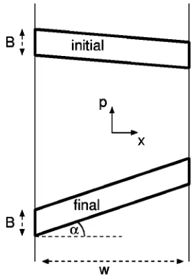
We approximate the bands in Fig. 3 by straight and nar-row strips in the shape of a parallelogram, disregarding any curvature. This is a good approximation in particular for the narrowest bands, which are the ones that determine the shot noise. Each band is characterized by a mean dwell time n共in units of 0). We disregard any variations in the dwell time within a given band, assuming that the entire band exits through one of the two leads after n iterations. 共We have found numerically that this is true with rare exceptions.兲
The case of a reflection band is shown in Fig. 5. The initial and final parallelograms have the same height, set by the width w⫽N/ M of the lead. Since the map is area
pre-serving, the base B of the two parallelograms should be the same as well. To calculate the band area A⫽Bw we assume
that the monodromy matrix M (xk, pk) does not vary
appre-ciably within the band at each iteration k⫽1,2, . . . ,n. An initial vector eជiwithin the parallelogram is then mapped after
n iterations onto a final vector eជf given by
e
ជf⫽Meជi,M⫽M共xn, pn兲•••M共x2, p2兲M共x1, p1兲, 共A1兲 with x1, p1 inside the initial parallelogram.
We apply Eq.共A1兲to the vectors that form the sides of the initial and final parallelograms. The base vector eជi⫽B pˆ is mapped onto the vector eជf⫽⫾w(xˆ⫹pˆtan␣), with␣ being the tilt angle of the final parallelogram. It follows that
B兩Mx p兩⫽w, hence
A⫽w2/兩Mx p兩. 共A2兲
We obtain the Fano factor F by a Monte Carlo procedure. An initial point x1, p1 is chosen randomly in lead 1 and iterated until it exits through one of the two leads. The prod-uctMof monodromy matrices starting from that point gives the area A of the band to which it belongs, according to Eq. 共A2兲. The fraction of points with A⬍1/M then equals
w⫺1兰0 1/M
A(A) dA⫽4F, according to Eq.共4.2兲.
To assess the accuracy of this procedure, we repeat the calculation of the Fano factor with initial points chosen ran-domly in lead 2 共instead of lead 1兲. The difference is about 5%. The dashed lines in Fig. 1 are the average of these two results.
1C.W.J. Beenakker and C. Scho¨nenberger, Phys. Today 85„5…, 37 共2003兲.
2O. Agam, I. Aleiner, and A. Larkin, Phys. Rev. Lett. 85, 3153 共2000兲.
3H.-S. Sim and H. Schomerus, Phys. Rev. Lett. 89, 066801共2002兲. 4R.G. Nazmitdinov, H.-S. Sim, H. Schomerus, and I. Rotter, Phys.
Rev. B 66, 241302共R兲 共2002兲.
[image:5.612.367.506.56.256.2]5P.G. Silvestrov, M.C. Goorden, and C.W.J. Beenakker, Phys. Rev.
FIG. 5. Phase space of a lead共width w) showing two areas共in the shape of a parallelogram兲that are mapped onto each other after
n iterations. They have the same base B, so the same area, but their
Lett. 90, 116801共2003兲.
6H. Schanz, M. Puhlmann, and T. Geisel, cond-mat/0304265共 un-published兲.
7
S. Oberholzer, E.V. Sukhorukov, and C. Scho¨nenberger, Nature 共London兲415, 765共2002兲.
8C.W.J. Beenakker and H. van Houten, Phys. Rev. B 43, 12 066 共1991兲.
9S. Oberholzer, Ph.D. thesis, 2001共unpublished兲.
10Ph. Jacquod, H. Schomerus, and C.W.J. Beenakker, Phys. Rev. Lett. 90, 207004共2003兲.
11E.B. Bogomolny, Nonlinearity 5, 805共1992兲. 12R.E. Prange, Phys. Rev. Lett. 90, 070401共2003兲.
13F. Borgonovi, I. Guarneri, and D.L. Shepelyansky, Phys. Rev. A
43, 4517共1991兲.
14F. Borgonovi and I. Guarneri, J. Phys. A 25, 3239共1992兲. 15A. Ossipov, T. Kottos, and T. Geisel, Europhys. Lett. 62, 719
共2003兲.
16F.M. Izrailev, Phys. Rep. 196, 299共1990兲.
17F. Haake, Quantum Signatures of Chaos共Springer, Berlin, 1992兲. 18Y.V. Fyodorov and H.-J. Sommers, Pis’ma Zh. Eksp. Teor. Fiz.
72, 605共2000兲 关JETP Lett. 72, 422共2000兲兴. 19M. Bu¨ttiker, Phys. Rev. Lett. 65, 2901共1990兲.
20T. Guhr, A. Mu¨ller-Groeling, and H.A. Weidenmu¨ller, Phys. Rep.
299, 189共1998兲.
21C.W.J. Beenakker, Rev. Mod. Phys. 69, 731共1997兲.
22R. Ketzmerick, K. Kruse, and T. Geisel, Physica D 131, 247 共1999兲.
23
The iterative procedure we found most stable was the bi-conjugate-stabilized-gradient routineF11BSFfrom the NAG共 Nu-merical Algorithms Group兲library.
24M.G. Vavilov and A.I. Larkin, Phys. Rev. B 67, 115335共2003兲. 25R.A. Jalabert, J.-L. Pichard, and C.W.J. Beenakker, Europhys.