Chemical transport model ozone simulations for spring 2001 over the western Pacific: Regional ozone production and its global impacts

Chemical transport model ozone simulations for

spring 2001 over the western Pacific: Regional ozone

production and its global impacts

Oliver Wild,1 Michael J. Prather,2Hajime Akimoto,1Jostein K. Sundet,3

Ivar S. A. Isaksen,3James H. Crawford,4 Douglas D. Davis,5 Melody A. Avery,4 Yutaka Kondo,6Glen W. Sachse,4 and Scott T. Sandholm5

Received 4 August 2003; revised 24 October 2003; accepted 6 November 2003; published 21 May 2004.

[1] The spatial and temporal variation in ozone production over major source regions in

East Asia during the NASA Transport and Chemical Evolution over the Pacific (TRACE-P) measurement campaign in spring 2001 is assessed using a global chemical transport model. There is a strong latitudinal gradient in ozone production in springtime, driven by regional photochemistry, which rapidly diminishes as the season progresses. The great variability in meteorological conditions characteristic of East Asia in springtime leads to large daily variability in regional ozone formation, but we find that it has relatively little impact on the total global production. We note that transport processes effectively modulate and thus stabilize total ozone production through their influence over its location. However, the impact on the global ozone burden, important for assessing the effects of precursor emissions on tropospheric oxidizing capacity and climate, is sensitive to local meteorology through the effects of location on chemical lifetime. Stagnant, anticyclonic conditions conducive to substantial boundary layer ozone production typically allow little lifting of precursors into the free troposphere where greater ozone production could occur, and the consequent shorter chemical lifetime for ozone leads to relatively small impacts on global ozone. Conversely, cyclonic conditions with heavy cloud cover suppressing regional ozone production are often associated with substantial cloud convection, enhancing subsequent production in the free troposphere where chemical lifetimes are longer, and the impacts on global ozone are correspondingly greater. We find that ozone formation in the boundary layer and free troposphere outside the region of precursor emissions dominates total gross production from these sources in springtime, and that it makes a big contribution to the long range transport of ozone, which is greatest in this season. INDEXTERMS:0345 Atmospheric Composition and Structure: Pollution—urban and regional (0305); 0365 Atmospheric Composition and Structure: Troposphere—composition and chemistry; 0368 Atmospheric Composition and Structure: Troposphere—constituent transport and chemistry;KEYWORDS: tropospheric ozone, western Pacific, meteorological variability

Citation: Wild, O., et al. (2004), Chemical transport model ozone simulations for spring 2001 over the western Pacific: Regional ozone production and its global impacts,J. Geophys. Res.,109, D15S02, doi:10.1029/2003JD004041.

1. Introduction

[2] Photochemical formation of ozone in the troposphere

from precursor species such as nitrogen oxides (NOx),

carbon monoxide (CO) and hydrocarbons leads to a degra-dation of local air quality [Haagen-Smit, 1952] and to a global increase in O3that leads to a global warming [Lacis

et al., 1990; Hansen et al., 1997]. The link between these regional and global impacts is becoming increasingly evi-dent [Hansen, 2002]. Ozone is also the principal source of tropospheric OH radicals and therefore controls the rate at which gases such as methane are oxidized [e.g.,Chameides and Walker, 1973;Crutzen, 1974; Thompson, 1992]. On a global scale, the photochemical production of O3 in the

troposphere generally dominates the stratospheric influx [Liu et al., 1980; Lelieveld and Dentener, 2000; Prather and Ehhalt, 2001]. While the production mechanisms are well known [e.g., Chameides and Walker, 1973; Crutzen, 1974; Logan et al., 1981], the magnitude, timing and 1

Frontier Research System for Global Change, Yokohama, Japan. 2

Earth System Science, University of California, Irvine, California, USA.

3

Department of Geophysics, University of Oslo, Oslo, Norway. 4_{NASA Langley Research Center, Hampton, Virginia, USA.} 5

School of Earth and Atmospheric Sciences, Georgia Institute of Technology, Atlanta, Georgia, USA.

6

Research Center for Advanced Science and Technology, University of Tokyo, Japan.

location of greatest O3 formation depend on the

meteoro-logical environment about the region of precursor emis-sions. Meteorological processes effectively modulate the chemical processing of O3through the amount of sunlight

and water vapor, the residence time in the boundary layer, the dilution and mixing of different precursors and their scavenging by clouds and precipitation, and the long-range transport and dispersion of the O3produced.

[3] In the polluted boundary layer, the lifetime of O₃to

chemical destruction and deposition is relatively short (days), but it remains longer than typical dynamical time scales (hours to days), and hence much of the O3formed

may be transported to cleaner environments. Atmospheric lifting processes associated with convection or frontal systems [Pickering et al., 1990; Bethan et al., 1998] are particularly important in controlling the global impacts of the O3formed as they raise it higher into the troposphere

where the lifetime to chemical destruction is longer (weeks to months). Transport of O3 precursors out of polluted

emission regions typically leads to slower but greater total O3production [Liu et al., 1987], and supplements

produc-tion from sources in the troposphere such as lightning. The export of short-lived precursors such as NOx is generally

inefficient [Horowitz et al., 1998] and subsequent O3

production in the free troposphere from boundary layer sources is therefore dependent on temporary storage as longer-lived NOy species and on the location and timing

of rapid vertical transport by convection. Chatfield and Delany [1990] provided contrasting examples of O3

pro-duction in biomass burning plumes undergoing delayed or immediate convective lifting, colorfully termed ‘‘cook-then-mix’’ and ‘‘mix-then-cook’’ scenarios, demonstrating very different impacts on regional and global O3. While

rapid boundary layer formation in stagnant conditions over polluted urban regions in the presence of strong sunlight and high temperatures may lead to a large buildup of smog O3,Sillman and Samson[1995] speculated that the impacts

on global O3, and hence on climate, may be less than in

overcast conditions where O3 buildup is small, but the

export of precursors is larger. The balance between regional and downwind production and its sensitivity to meteorology is thus important both for assessing the impacts of surface emissions on air quality and climate, and for understanding how global or regional climate change may affect these impacts in the future.

[4] This study uses the extensive set of measurements and

analysis from the NASA Transport and Chemical Evolution over the Pacific (TRACE-P) measurement campaign held in spring 2001 [Jacob et al., 2003] as a case study to examine the meteorological factors controlling production of O3

from fossil fuel sources over East Asia. Outflow of pollution from rapidly developing countries around the Pacific Rim is known to influence tropospheric O3on a hemispheric scale,

and has the greatest effects in springtime [Berntsen et al., 1996;Jacob et al., 1999;Mauzerall et al., 2000;Wild and Akimoto, 2001;Bey et al., 2001]. The meteorology of the region in spring is characterized by strong frontal activity which lifts pollution into the path of strong westerly winds which may carry it across the Pacific. This transport is consequently episodic in nature [Yienger et al., 2000], as the passage of successive low pressure systems interlaces polluted continental ou with cleaner, marine air and

with dry air from the stratosphere descending in trailing anticyclones [Carmichael et al., 1998]. The meteorological processes leading to this variability in outflow also strongly influence O3production directly via their impacts on mixing

processes, humidity, photolysis rates and scavenging of precursors, providing ideal conditions for study of variabil-ity in O3production and its global impacts.

[5] While previous studies have characterized the

pro-duction and export of O3from East Asia on a seasonal or

annual basis, this study uses the day-to-day variations in weather to identify the meteorological factors controlling the buildup of tropospheric O3. By following the emission

of O3precursors each day from a specified region

indepen-dently, we show how the different meteorological condi-tions affect local versus regional production and thus how the synoptic weather patterns control the net impact of emissions on global tropospheric O3. The principal aims

of the paper are to quantify the contributions of East Asian emissions to global O3during springtime, to relate these to

the meteorological conditions over the source region, and thus to examine how meteorological mechanisms control the balance between local air quality and global climate forcing.

[6] In section 2, we evaluate the performance of the

model used in this study against O3 tendencies derived

from TRACE-P observations. This campaign provided extensive observational data from two aircraft operating in the region with sufficient detail to allow thorough testing of current photochemical theory [Cantrell et al., 2003]. We examine the regional production of O3 from East Asia

during the spring of 2001 in section 3. We then focus on the daily variability in O3 production from each day’s

emissions in section 4, exploring its dependence on mete-orological conditions, and noting generally opposite impacts on air quality and climate forcing. We conclude by testing the sensitivity of production to specific meteoro-logical variables, and identifying potential biases in this study.

2. Chemical Transport Model Ozone Production

[7] This study uses the Frontier Research System for

Global Change (FRSGC) version of the University of California, Irvine (UCI), global chemical transport model (CTM), described byWild and Prather[2000]. The model is run at T63 resolution (1.91.9), with 37 eta levels in the vertical, and is driven by 3-hour meteorological fields for spring 2001 generated with the European Centre for Medium-Range Weather Forecasts (ECMWF) Integrated Forecast System (IFS). The configuration of the model and meteorological data used in these studies is described in more detail byWild et al.[2003] and is presented with an evaluation of the O3simulation during the TRACE-P period

against observations from aircraft, ozonesondes, and satel-lite. The model uses a linearized stratospheric chemistry for O3[McLinden et al., 2000] and calculates a reasonable net

flux of O3 from the stratosphere to the troposphere of

557 Tg yr 1. With this treatment, the model is able to capture the short-term variations in total column O3which

the Pacific are reproduced very well [Wild et al., 2003], although there is a tendency to overestimate the total O3

column at 45N by about 12% compared with columns from the TOMS satellite instrument, and to overestimate boundary layer O3near polluted continental regions by an

average of 12 ppbv at ozonesonde locations. Further model evaluation and assessment of the representativeness of the TRACE-P measurements is presented byHsu et al.[2004]. [8] To evaluate the CTM simulation of O₃ production

over the western Pacific, we compare the instantaneous net chemical production of O3 sampled from the model fields

at 1-min intervals along the flight tracks of the NASA DC-8 and P-3B aircraft during the TRACE-P campaign with those derived fro otochemical steady state box

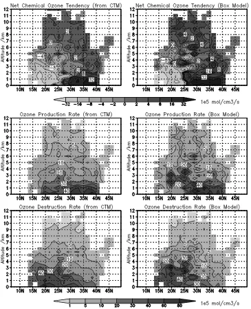
model calculations driven by observed precursor concen-trations and photolysis rate coefficients using the Georgia Tech/NASA Langley box model [Crawford et al., 1999]. Figure 1 shows the mean latitude-height tendency for O3for

all flights over the western Pacific region, binned onto the horizontal grid of the model (190 km) and onto 500-m levels in the vertical. Where key observational variables constraining the box model are unavailable and the O3

tendency cannot be calculated, the CTM value is omitted so that the sampling is identical. Ozone destruction domi-nates in the lower troposphere south of 27N and below 6 km in clean, marine air masses; north of this region, there is strong production in the lower troposphere in the conti-nental outflow from China and Korea and from sources over

Figure 1. Net chemical O3tendency (105molecules cm 3s 1, top) over the western Pacific (west of

145E south of 30N, west of 160E north of 30N) (left) from the CTM and (right) from steady state calculations constrained by aircraft measurements along flight tracks during the TRACE-P campaign. (bottom) Gross O3production and destruction rates with a different color scale used. See color version of

Japan. This clear separation into two distinct regimes is similar to that found during the PEM-West B campaign in 1994 [Crawford et al., 1997], and reflects both the location of major sources and the key meteorological boundaries in spring. There is significant O3 production in the upper

troposphere over the whole region, greatest at about 10 km, similar to that found 3 weeks earlier in 1994 during the PEM-West B campaign [Crawford et al., 1997] and 1 month later in 1998 during the BIBLE-T campaign [Miyazaki et al., 2003]. The gross production rate, defined as the sum of the rates of NO reaction with modeled peroxy radicals following Crawford et al. [1997], is shown sepa-rately in Figure 1 (bottom). While boundary layer produc-tion is reasonably well matched, there is a significant underestimation of formation in the middle and upper troposphere relative to the constrained model, which con-tributes to a mean underestimation of net production of

30% in this region. The destruction rate matches the constrained model more closely except in the pollution plumes sampled between 2 and 6 km. The locations of many of the plume features are captured, but the magnitude of formation and destruction in these layers is typically underestimated as they fall below the grid scale of the model.

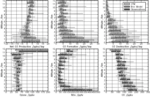
[9] The simulations can be compared in more detail by

considering the statisti stributions of the aircraft and

model data along the flight tracks averaged over 1-km altitude bins; see Figure 2. In the lower troposphere, the net production is reasonably well matched, although the high-end distributions are somewhat low as plume condi-tions cannot be reproduced. Between 2 and 5 km, there is slow net destruction, and both formation and destruction rates remain large; above 5 km, destruction is slow, and formation dominates. The profile of the main O3precursor

species, NOx, is reproduced well in shape, but mean

abundances are consistently underestimated by about 35%. Consequently, while the gross O3destruction rate is

simu-lated well, the gross formation rate is on average 20% low. The CTM does not capture the variability in O3formation

driven by the presence of plumes, which also contributes to this bias. The O3 profile reveals an overestimation in the

boundary layer, but the mean abundance of O3is 9% low in

the 6 – 10 km region, consistent with underestimated pro-duction. The larger modeled variability in O3in this region

indicates that stratospheric influence also makes a signifi-cant contribution here. The principal oxidation products of NOx, nitric acid and peroxyacetyl nitrate (PAN), are

repro-duced reasonably well in the free troposphere, but are overestimated by about 70% in the boundary layer. This may reflect poor simulation of regional emission or depo-sition processes, but it may also be attributed to overesti-mation of O3 and hence OH production in the polluted

boundary layer over source regions, leading to oxidation of NOxwhich is too rapid.

[10] The photolysis frequencies of O₃ and NO₂, which

play important roles in O3 formation and destruction, are

generally well simulated, with mean values 2% and 13% above those observed, respectively. This reflects uncertain-ties in the simulation of cloud cover as well as in calculation and measurement error, and is similar to comparisons from previous measurement campaigns [Shetter et al., 2003]. Specific humidity is generally reproduced well in the meteorological fields at the surface and in coastal regions at ozonesonde stations [Wild et al., 2003]. It is overesti-mated by an average of 2% compared with diode laser hygrometer measurements from the DC-8 aircraft [Podolske et al., 2003] and by 6% compared with the composite measurements used to drive the box model, heavily biased by overestimation at 5 – 8 km over the ocean at 30 – 35N. This may be partly responsible for overestimation of OH and HO2, which are on average 9% high compared with the

box model. Note, however, that this falls well within the 30% 1-s error estimated for the box model calculations [Davis et al., 2003] and that the error in the CTM simulation is likely to be larger. However, OH is 60 – 80% higher than the aircraft observations in the middle and upper tropo-sphere, indicating a significant discrepancy between the measurements and current understanding of photochemistry that remains to be resolved. The overestimation of HOxwith

the box model also highlights the uncertainty in the mea-surement-derived O3tendencies.

[11] The overestimation of O3and NOyin the boundary

layer and underestimation of NOx in the free troposphere

suggests either that there is insufficient vertical lifting of O3

and precursors out of the boundary layer, or that O3 is

produced on timescales which are too short close to source regions. The simulate ributions of CO have been

evaluated elsewhere [Kiley et al., 2003; Hsu et al., 2004], and though abundances are underestimated here by an average of 6%, no significant vertical bias suggesting insufficient lifting is evident; see Figure 2. It is therefore likely that the underestimation of O3 production in the

middle and upper troposphere relative to the constrained model is due to shorter model timescales for production in source regions, caused by neglecting the impact of aerosol effects on photolysis rates [Martin et al., 2003;Bian et al., 2003;Tang et al., 2003], by simplifications of hydrocarbon oxidation and omission of heterogeneous processes in the chemical scheme, and by the effects of coarse model resolution on nonlinear HOx/O3/NOx chemistry. The

assumption of instantaneous mixing within a model grid box is known to cause overestimation of O3 production

[Sillman et al., 1990;Chatfield and Delany, 1990;Jacob et al., 1993], and the consequent reduced export of precursors may lead to reduced production downwind. The implica-tions of resolution for the present study will be addressed further below.

[12] The uncertainties in this comparison are clearly large

and originate from source strengths and their variability, from sampling the relatively coarse resolution CTM data in the presence of small-scale features such as outflow plumes and cloud cover, and from the assumptions used in deriving instantaneous production in the two models. Nevertheless, the magnitudes and patterns of formation and destruction agree sufficiently well to improve confidence in our ability to simulate O3 production in the troposphere, while also

pointing to potential biases in the model simulations.

3. Regional Ozone Production

[13] We first consider the temporal and spatial variations

in O3 production over the east Asian region during the

TRACE-P campaign period. The daily net O3 production

rate in the boundary layer (below 750 hPa,2 km) over the extended region (5– 45N, 95– 150E) for February to April 2001 is shown in Figure 3. The mean net production rate is 246 Gg d 1, and shows little trend over the period, although the day-to-day variability is large, about 28 Gg d 1 (1s). The total net production in the regional boundary layer over the period is 21.9 Tg. The mean net production rate through the depth of the troposphere is 320 Gg d 1, indicating that free-tropospheric production is responsible for about 23% of the total net production over the region. This is in reasonable agreement with earlier studies [Pierce et al., 2003] which estimated a mean production rate of 370 Gg d 1between 7 March and 12 April 2001, over a domain slightly larger than that used here; we find a production rate of 340 Gg d 1 over the same period. Although we choose not to diagnose the gross flux of O3

from the stratosphere on the grounds that it is resolution-dependent and thus not a useful measure of stratosphere-troposphere exchange [Hall and Holzer, 2003], we find that about 30% of the O3 over the region is of stratospheric

origin, dropping to 20% in the boundary layer, consistent with earlier findings [Pierce et al., 2003].

[14] The net O3 production rate in the boundary layer

over China, the closest source region to the measurements made during TRACE-P, is shown separately in Figure 3, and accounts for just over half of the net regional

produc-Figure 3. Daily net chemical O3tendency in the boundary

tion, 134 Gg d 1. The increasing photochemical activity over this more northerly part of Asia during springtime leads to a clear trend, with O3production increasing by an

average of 0.70 Gg d 2. This trend appears stronger in the first half of the period. The residual production from east Asia outside China decreases during the period, as produc-tion is dominated by biomass burning sources which peak in February and March; consequently the relative importance of sources in China on total regional production increases strongly over the period, from 45% at the beginning of February to 63% by the end of April. The variability in the detrended daily production is 15% (1s), and reflects differ-ences in the meteorological variables that modulate O3

production, in particular cloud cover, temperature and boundary layer residence time. This will be explored in more detail in section 4.

[15] In contrast, net boundary layer O₃ production over

Europe is found to average 125 Gg d 1 over the same period, and over the United States is 187 Gg d 1; see Table 1. Both regions exhibit larger temporal trends, 2.0 Gg d 2over Europe and 3.0 Gg d 2over the United States.

[16] To investigate the trend in net O₃production over the

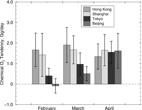
spring season in more detail, we examine production over large, heavily populated metropolitan regions in East Asia, focusing on Hong Kong, Shanghai, Beijing and Tokyo. Figure 4 shows the monthly mean production rate in the boundary layer over each 22region, together with its day-to-day variability. Over the south of the region, O3

production is strong and the seasonal increase is weak; there is a decrease in production over Hong Kong in April caused by a decrease in biomass burning sources from neighboring regions and by increased cloud cover. In contrast, more northerly regions such as Beijing and Tokyo show rapidly increasing photochemical activity due to longer daylight hours and higher temperatures. Ozone formation is suffi-ciently slow in February that total boundary layer production is small, and for Beijing we find a small net destruction. Consequently there is a strong latitudinal gradient in O3

production in February that disappears by April. A signifi-cant gradient is still present during the March time period of the TRACE-P campaign.

4. Regional Versus Global Production

[17] Boundary layer O3formation from regional

precur-sor emissions occurs on relatively short timescales, and is important in controlling regional air quality. However, the impacts of these surface emissions on the global O3budget,

important for assessing effects on climate and tropospheric oxidizing capacity, is also dependent on continued produc-tion in the free troposphere from transported precursors, which occurs on longer timescales. The relative importance of regional and downwind production for the global O3

budget is strongly dep on meteorological processes,

and has not been clearly characterized. The sensitivity of the large-scale impacts on O3to the occurrence and timing of

deep convection has been highlighted by Chatfield and Delany[1990], and the sensitivity of production in polluted air masses from North America to dilution and the timing of lifting processes over the North Atlantic has been explored byWild et al. [1996]. Here we quantify the importance of O3 production in the free troposphere from fossil fuel

sources in East Asia, and examine how meteorological processes control its variability. The aim is to investigate the evolution of the chemical outflow over the Pacific in springtime and its sensitivity to meteorology and hence to contribute to a better understanding of the global impacts of this region.

[18] We determine the influence of polluted metropolitan

regions by making a small perturbation (20%) to the fossil fuel and industrial sources of NOx, CO, and nonmethane

hydrocarbons over a single region for 1 day. We follow the impacts of this perturbation over the following 5 weeks by comparing this simulation with a control run with the standard emissions. Separate perturbations are performed for each of the 31 days in March and for each of the four metropolitan regions defined above. The responses pre-sented here are scaled by a factor of 5 to provide a linear estimation of those from the full emissions for each day. The primary diagnostics presented are the gross production of O3 and the perturbation to O3 abundance. The gross

production provides some insight into the timescales and location of chemical formation. However, the impacts of precursor emissions are driven principally by the additional O3abundance. This is the more useful diagnostic, since the

lifetime of O3varies greatly with latitude and altitude, and

may be sufficiently short compared to transport that much does not escape the region of formation. Both these diag-nostics are considered over three distinct volumes: the regional boundary layer (RBL) over the metropolitan re-gion, the distant boundary layer (DBL) comprising the boundary layer over the rest of the globe, and the free troposphere (FT). These three volumes together cover the Table 1. Net Boundary Layer O3 Production, February – April

2001

Region Domain Production, Gg d 1_{Trend, Gg d} 2

East Asia 5– 45N, 95– 150E 246 0.1 China 22– 45N, 100– 125E 134 0.7 Europe 35– 67N, 10W – 30E 125 2.0 United States 28– 49N, 124– 70W 187 3.0

Figure 4. Net chemical O3 tendency over four large

global troposphere. To reduce the computational require-ments of this study, the horizontal resolution of the model is reduced to T21 (5.6 5.6). While this increases the effective size of the metropolitan regions considered, the additional spatial averaging may also lead to overestimation of regional O3 production, as noted above. We find an

increase in O3formation in the East Asian boundary layer in

March of about 10%; sampled along the aircraft flight tracks there is increased production below 2 km, reduced produc-tion between 2 and 8 km, and very little change in the upper troposphere, consistent with the changes in chemical time-scales expected due to resolution.

4.1. Evolution of Ozone Production

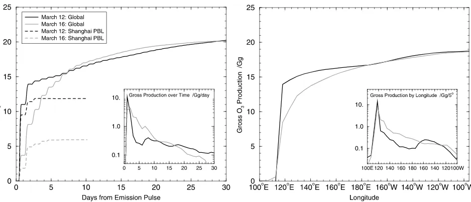
[19] Figure 5 shows contrasting examples of regional and

global O3 perturbations following emissions pulses over

Shanghai. The meteorological conditions on these days and the additional gross O3production over the first 3 days are

shown in Figure 6. On 12 March, the region was dominated by a high pressure system with clear skies and low humid-ity, leading to rapid boundary layer O3production.

Large-scale subsidence prevented lifting of precursors and outflow of air was principally at low altitudes; direct export of O3

and further production from exported precursors both con-tribute to a boundary layer enhancement outside the region. Significant eastward transport and lifting do not occur until after the third day, by time most of the additional

precursor NOxhas been removed, and subsequent

produc-tion above the boundary layer accounts for less than 10% of the total O3production. After the first week, about 60% of

the additional O3is in the midtroposphere (750 – 400 hPa),

but only about 10% reaches the upper troposphere (above 400 hPa), mostly in a single lifting event ahead of a cyclone northeast of Japan on 18 March (day 7). The perturbation decays quickly in the midtroposphere due to chemical destruction and subsidence, with an e-folding decay time of 4 weeks, but more slowly elsewhere. Interestingly, boundary layer O3remains steady over the second and third

weeks, as chemical destruction and deposition to the ocean is counterbalanced almost equally by subsidence from the troposphere and by additional formation from transported precursors.

[20] In contrast, on 16 March the area was under heavy

cloud cover close to a region of cyclogenesis, and boundary layer O3formation was greatly reduced. Regional

produc-tion peaked on the second day, and total producproduc-tion was only half that of 12 March. However, convection associated with the cloud cover lifted precursors into the free tropo-sphere, and significant additional formation, almost 40% of the total, occurs there on longer time scales. The maximum global O3perturbation does not occur until day 7,

empha-sizing the slower mean chemical formation rates compared with 12 March, but the magnitude is very similar. A larger proportion of the O3change (25 – 30%) occurs in the upper

troposphere and is strongly dominated by downwind pro-duction, in contrast to 12 March. However, O3 in the

midtroposphere decays more quickly in this case, with a lifetime of 3 weeks, reflecting different meteorological impacts over the Pacific and beyond, and the global perturbation decays at a slightly faster rate.

[21] Although the precursor emissions in these two cases

are the same and the integrated O3 perturbations are very

similar (within 2% over the first month), the O3responses

are quite different. In the former case regional production is rapid and O3 is then transported to the global atmosphere,

while in the latter case production is slow, transport of precursors is greater, and total formation is dominated by tropospheric production outside the region. These cases are representative of the cook-then-mix and mix-then-cook scenarios of Chatfield and Delany [1990], although the lifting processes here are not as strong as in the tropical regions of South America that they considered. The com-bination of lifting processes present over this region is revealed for the 16 March case in Figure 6. Convective lifting of precursors on the first day leads to enhancement of O3 formation at 350 hPa, but slower lifting ahead of a

frontal system on the third day leads to a rising band of enhanced formation in the lower troposphere reaching 140E.

[22] The evolution and location of additional gross

pro-duction is shown in Figure 7. While propro-duction in the regional boundary layer is limited to 3 – 4 days due to transport of precursors out of the region, subsequent for-mation in the troposphere continues for more than a month. Initially this is restricted close to the source region; the 3-day period shown in Figure 6 represents 70% of the total formation for 12 March, and 50% for 16 March. The greater direct export of precursors on 16 March leads to much greater production outside the region in the first

Figure 5. Additional mass of O3from 1 day’s emissions

Figure 6. Column- and latitude-mean additional gross O3 production (pptv) over the first 3 days

following 1 day’s emissions of precursors from Shanghai on (left) 12 March and (right) 16 March. Mean sea level pressure (grey contours) and cloud optical depth (shading) at the end of the first day are shown in the top panels. See color version of this figure in the HTML.

Figure 7. Cumulative additional O3 formation (left) with time and (right) with longitude following

week, most of which occurs over the western Pacific. The longitudinal variation in Figure 7 suggests that up to 18% of the formation for the 16 March case occurs between 125E and 150E in the region sampled during the TRACE-P campaign but only 6% for the 12 March case. However, in both cases, more than 25% of formation occurs after the first week, and almost 20% occurs east of the dateline. For the 16 March case, O3 formation drops off steadily with time

and distance from the source, and further formation is governed by longer timescales in the upper troposphere. For the 12 March case, on the other hand, almost 10% of the total formation occurs in the lower troposphere over the eastern Pacific, following subsidence and thermal decom-position of PAN during the second week. Note, however, that this region remains a net sink for O3, as destruction of

transported O3 formed earlier exceeds this additional

for-mation. This is in good agreement with previous studies of the central/eastern North Pacific region by DiNunno et al. [2003].

[23] Despite the different regional responses, the net

global responses are of similar magnitude, suggesting that it may be possible to parameterize the global impacts on O3

based on regional emissions alone. However, this is not always the case, and the global impacts can sometimes differ substantially, as we shall demonstrate below.

4.2. Gross Production

[24] We calculate gross O₃ production over the source

region and over the globe in the first month following each

pulse of emissions. Figure 8 shows the gross additional formation following pulses for each day of March over Shanghai and over Tokyo. For each region emissions are the same each day; while NOxemissions over the two regions

are comparable, CO emissions over eastern China are almost 5 times larger than over Japan due to the prevalence of coal and biofuel burning. The same experiments were performed for Beijing and Hong Kong; the impacts are similar to those over Tokyo and Shanghai, respectively, and the total production and variability are presented separately in Table 2.

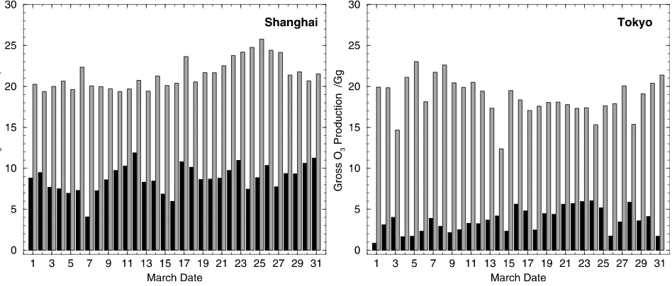
[25] Ozone formation from local sources over the

Shang-hai region is more than twice that over Tokyo, but total global formation is only about 15% greater. In both cases, formation downwind of the source region dominates global formation, with regional production accounting for about 40% of the total from Shanghai, but less than 20% from Tokyo. The lower proportion for Tokyo reflects both longer timescales for chemical formation due to lower temper-atures and shorter daylight hours and shorter air mass residence times due to different meteorological conditions. Stagnant, anticyclonic conditions are more common over eastern China, and lead to greater production and less variability than the changeable conditions associated with frontal passage over Japan. Both regions show a greater daily variability in regional production (20 – 40%) than in global production (8 – 12%), suggesting that regional mete-orology has a relatively small impact on total gross produc-tion, and exerts more control over the location of formation

Figure 8. Additional gross O3production over one month over the source region (black) and over the

globe (grey) following 1 day’s emissions of precursors from Shanghai and from Tokyo for each day of March.

Table 2. Ozone Production From 1 Day’s Emissions of Precursors in March 2001

Region

Emissions Gross Production Mean Burden

NOx,

103_{kg N 10}CO,6_kg Region,₁₀6_{kg 10}Globe,6_{kg in region}Fraction Region,₁₀6_kg Globe,₁₀6_kg

Beijing 730 19.5 2.4 ± 1.3 16.9 ± 2.6 0.14 0.03 ± 0.15 5.67 ± 1.39

Tokyo 780 4.3 3.6 ± 1.5 18.7 ± 2.3 0.19 0.29 ± 0.33 7.77 ± 1.43

Shanghai 720 21.1 8.8 ± 1.7 21.5 ± 1.8 0.41 1.86 ± 0.96 5.41 ± 0.80

via the chemical and dynamical timescales than over its total magnitude.

[26] Downwind production in the troposphere is at least

as important from the more northerly source regions of Tokyo and Beijing as from Shanghai and Hong Kong, despite the lower regional production. However, the longer timescales for chemical formation suggest that the more southerly regions will make a bigger contribution to total production over the western Pacific in the region sampled during the TRACE-P campaign, while the more northerly sources dominate at greater distances.

4.3. Mean Burden

[27] The impacts of precursor emissions are principally

driven by the additional abundance of O3rather than by the

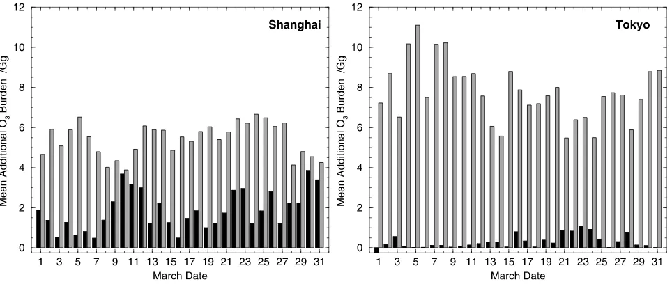
gross production. We therefore consider the additional mean global burden over the first month, broadly representative of the radiative impacts over the period, and the mean regional burden averaged over 3 days, reflecting the impacts on air quality, see Figure 9. This reveals the importance of the location and lifetime of the O3formed.

[28] For Shanghai, the variability in the regional burden is

much larger than that in production. Fair-weather, anticy-clonic conditions favoring O3 formation, such as that on

10 – 12 March, are often associated with relatively stagnant conditions, and O3buildup is consequently large. However,

suppression of lifting processes in these conditions leads to export of O3 and precursors principally in the boundary

layer, where the lifetime of O3 is shorter than at higher

altitudes, and where additional production from exported precursors is relatively inefficient. The impact on the global burden is consequently less in these stagnant conditions than at other times. This confirms speculation by Sillman and Samson[1995], based on studies of O3production in a

one-dimensional model, that the global burden of O3may

be affected to a greater extent by surface emissions when localized high O3does not occur.

[29] Over Tokyo, the frequent passage of cyclonic

sys-tems in March does n w much buildup of O3 from

regional emissions. However, the impacts on the global burden are almost 50% larger than over Shanghai, despite lower gross production. This is because formation and destruction are sufficiently slow that more O3 reaches

higher altitudes and latitudes where the lifetime is longer. The higher CO emissions over Shanghai are responsible for about 40% of the global O3perturbation, and 25% of the

regional perturbation, suggesting that Tokyo may have more than twice the impact on the global O3 burden given the

same emissions. The greater mean global burden would suggest that these northerly fossil fuel sources have a greater impact on climate forcing through O3 than regions

such as Shanghai or Hong Kong, although this may be offset by the reduced contribution of O3at higher latitudes

to total forcing [Roelofs et al., 1997]. A full assessment of the climate impacts would require a detailed calculation of radiative forcing taking into account the location of these changes and inclusion of the indirect effects on tropospheric methane.

4.4. Ozone Production Efficiency

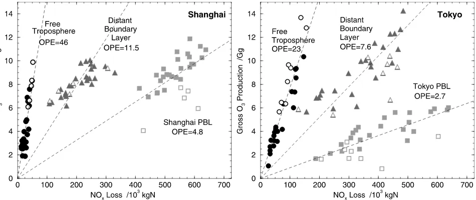
[30] To highlight the importance of the balance between

chemical and dynamical timescales, we consider the loca-tion and producloca-tion efficiency of O3 formed from each

day’s emissions. Figure 10 shows the gross production of O3 against the NOx lost for each pulse over the regional

boundary layer (Shanghai or Tokyo), the distant boundary layer, and the free troposphere. The global production is the sum of the production in these three domains, and the total NOx loss is the same in each case and is equal to the

additional emissions. The production efficiency is defined here as the gross production of O3per molecule of NOxlost,

as fromLiu et al.[1987], and loss of NOxdoes not include

temporary conversion to PAN.

[31] For each source region, the O₃ production values

cluster quite closely along lines representative of the O3

production efficiency for that domain, and mean production efficiencies are labeled in Figure 10. While there is a small spread in efficiencies reflecting different conditions, the

Figure 9. Mean additional mass of O3following each day’s emissions of precursors from Shanghai and

Tokyo, showing the additional O3over the source region (averaged over 3 days, black) and over the globe

values are sufficiently different over the domains consid-ered, typically a factor of 10 between the polluted boundary layer and the free troposphere, that the clusters remain quite distinct. Comparing the mean O3production and NOxloss

over each domain we find that about 40% of the gross O3

production over Shanghai occurs in the boundary layer from about 70% of the NOxemitted. Respectively 40% and 20%

of the production occur in the distant boundary layer and free troposphere, where production efficiencies are higher. Chemical timescales are sufficiently rapid that the boundary layer dominates removal of NOx, and only an average of 4%

reaches the free troposphere. Note, however, that the coarse model resolution used in these simulations may lead to a systematic bias in these conditions, with an underestimation of NOxexport as seen in section 2. Over Tokyo, 20% of the

production occurs in the boundary layer from 50% of the NOx emitted, with another 50% in the boundary layer

outside the source region. Slower chemical production and shorter dynamical timescales lead to a much greater vari-ability in boundary layer NOxremoval, and an average of

10% reaches the free troposphere. The O3 production

efficiencies over each domain are about half those over Shanghai, consistent with slower photochemical formation. However, the total production is similar due to the different distribution of production between the domains. This emphasizes the important role that transport of precursors plays in controlling gross O3production.

[32] Days with heavy daytime cloud cover (optical depth

greater than 10) are highlighted with unfilled markers in Figure 10. These typically have lower production efficien-cies in the regional boundary layer due to the increased cloud cover, but slightly higher production efficiencies in the free troposphere. Boundary layer NOxloss is less than

average due to the lower abundance of OH, and a greater proportion of the NOx is lifted into the troposphere by

convective processes, where total production is about a

factor of two greater. Consequently, these changes in time-scales shift some O3production out of the boundary layer

into the free troposphere, but do not alter the gross produc-tion or the mean burden greatly. Comparing the 5 days of heavy cloud cover over Shanghai with 10 largely cloud-free days, we find an increase in gross production of 5% and an increase in mean burden of 10%, suggesting that the impact on global O3may be larger on overcast days than in

fair-weather conditions.

4.5. Sensitivity to Meteorology

[33] To investigate the sensitivity of regional and global

O3production to meteorological processes, we consider the

changes to the conditions over Shanghai on 16 March required to reproduce the additional O3found on 12 March.

Convection, rainfall and cloud optical depth over Shanghai are removed for 16 March, and the temperature, humidity, boundary layer height and the O3column used in

calculat-ing photolysis rates are set to approximate the fair-weather values of 12 March for both emission pulse and control run. With all changes applied, global production is 15% greater than on 12 March, reflecting the effects of differing transport patterns and residence times, which were not altered.

[34] By altering each variable in turn, and neglecting the

coupling between them, we estimate that 60% of the difference in regional production is due to cloud cover suppressing photolysis rates, 20% is accounted for by reduced dilution of precursors due to the lower boundary layer height, and 15% is due to suppressed convection preventing lifting of precursors. The remaining 5% is dominated by increased temperature, but also reflects reduced humidity and total O3 column. Suppressing

con-vection reduces the global production by about 20%, reflecting the greater production efficiency per molecule of NOx in the free troposphere, but reduces the additional

Figure 10. Gross production of O3and loss of NOxfrom 1 day of emissions over (left) Shanghai and

global burden of O3 by 45% due to the short lifetime of

O3in the boundary layer. Removing the impact of clouds

on photolysis rates increases global production by about 15%, with 60% greater boundary layer production bal-anced against 5% less production elsewhere due to lack of enhancement in photolysis rates above clouds, and to reduced export of precursors due to shorter production time scales. The resultant impact on the global burden is very small, as these effects cancel. Increasing the boundary layer mixing height, appropriate to the fair-weather con-ditions on 12 March, causes an increase in global produc-tion of almost 40% as it provides an alternative method of lifting precursors into the free troposphere. However, no attempt has been made in this sensitivity study to keep the conditions dynamically consistent, and the stagnation and subsidence on 12 March prevent precursors exported by this mechanism from being carried away to regions of higher production efficiency. This interaction of dynamical processes emphasizes the need for boundary layer turbu-lence to be fully consistent with the large-scale dynamics to correctly simulate production of O3 in the free

tropo-sphere. Nevertheless, this sensitivity study demonstrates that the clear-sky conditions which strongly influence regional O3 production may have little impact on the

global abundance of O3, and that these global impacts

are most strongly influenced by lifting processes.

5. Conclusions

[35] We have explored the magnitude and patterns of O3

production from continental emissions over East Asia in springtime using a global CTM. The strengths and weak-nesses in the simulation of regional O3 production are

demonstrated by comparing it with values derived from observations during the NASA TRACE-P measurement campaign. The latitudinal and altitudinal variations in pro-duction and destruction are well simulated, although there is a tendency to underestimate net production in the upper troposphere and to overestimate it in the polluted boundary layer, suggesting that the timescales for production in the model are too short. High production and destruction rates are found in continental outflow regions, but the magnitudes are not reproduced well where small-scale pollution plumes occur at or below the model resolution.

[36] We present an O₃budget for East Asia in springtime,

finding relatively constant production over the season. However, we note that this masks an increase from north-east Asian sources, due to increasingly efficient photochem-ical formation, and a decrease over southeast Asia as the peak in biomass burning emissions has passed. Over eastern Asia, we note a strong latitudinal gradient in O3production

from large urban sources in February which diminishes during springtime and vanishes by April.

[37] We demonstrate that O₃production over major east

Asian source regions is highly variable, and is largely governed by meteorological processes, as previous studies over other regions have found [e.g.,Jacob et al., 1993]. On a global scale, we find that regional meteorological varia-tions have much less impact on the global production than on the regional production of O3, but that the net burden of

O3 is more dependent on them due to the variation in

location of production. , stagnant, anticyclonic

con-ditions greatly favor regional O3production which may lead

to significant pollution episodes, but reduced export of precursors supporting subsequent production and little lift-ing of the O3formed leads to short O3lifetimes and small

global impacts. In cool, cloudy conditions both the regional formation rate and the efficiency of production from pre-cursors are reduced, but shorter boundary layer residence times and lifting of O3 and its precursors by convection

associated with cloud cover enhances both the efficiency of production and the lifetime, and the global impacts are typically larger than in fair-weather conditions. We suggest that there is often a balance between the timescales for formation and for transport which buffers the total produc-tion but that the consequent variaproduc-tion in the locaproduc-tion of production may have a large impact on the chemical lifetime of the O3formed. The impacts on the global burden

of O3, important for assessment of climate effects, are more

sensitive to this balance. Attempts to estimate global impacts on O3based on regional export of precursors would

therefore greatly benefit from some consideration of the altitudinal distribution of expected O3formation.

[38] Understanding the chemical evolution of continental

outflow from Asia formed one of the objectives of the TRACE-P campaign. We find that gross chemical produc-tion in the troposphere away from the source region exceeds production in the regional boundary layer for each of the four 500-km square metropolitan regions considered. While the balance between regional and distant production is depen-dent on the size of the region considered, production outside the regional boundary layer remains important in all cases studied here and is greater when source regions are covered by cloud than when clear, anticyclonic conditions prevail. The contrast in spring weather between eastern China and Japan leads to the greater importance of remote production downwind of Tokyo than downwind of Shanghai, even though formation rates over the northwestern Pacific may be less due to the longer chemical timescales involved. The longer lifetime of O3 from these more northerly source

regions leads to a greater impact on the global burden, despite the smaller gross production that occurs.

[39] What biases are present in these results? The

rela-tively coarse resolution of the model used here is shown to lead to overestimation of production in the boundary layer and underestimation in the free troposphere, and hence both the importance of free tropospheric production and the meteorological impacts on the global burden may be larger than suggested here. The simple bulk mixing approach to boundary layer turbulence may also lead to overestimation of regional production [Wild et al., 2003]. Dust aerosol from northern and western China, maximum in spring, and black carbon from high levels of wintertime coal-burning both lead to significant reduction in photolysis rates, and may be expected to reduce regional O3production. Heterogeneous

chemical processes on the surface of these aerosol may also influence production [Jacob, 2000]. Our conclusions re-garding the global impacts on O3are also sensitive to the

chemical treatment of PAN in the model, which is respon-sible for much of the remote O3formation. Despite these

inadequacies, we demonstrate the strong link between regional meteorological processes and O3 production, and

mechanisms controlling O3transport also affect its chemical

production and lifetime.

[40] Acknowledgments. This work was supported by the NASA Tropospheric Chemistry Program as part of the TRACE-P mission. The ECMWF-IFS forecast data were generated under Special Project SPNOO3CL at the ECMWF.

References

Berntsen, T., I. S. A. Isaksen, W. C. Wang, and X. Z. Liang (1996), Impacts of increased anthropogenic emissions in Asia on tropospheric ozone and climate,Tellus, Ser. B,48, 13 – 32.

Bethan, S., G. Vaughan, C. Gerbig, A. Volz-Thomas, H. Richer, and D. A. Tiddeman (1998), Chemical air mass differences near fronts,J. Geophys. Res.,103, 13,413 – 13,434.

Bey, I., D. J. Jacob, J. A. Logan, and R. M. Yantosca (2001), Asian chem-ical outflow to the Pacific: Origins, pathways and budgets,J. Geophys. Res.,106, 23,097 – 23,114.

Bian, H., M. J. Prather, and T. Takemura (2003), Tropospheric aerosol impacts on trace gas budgets through photolysis, J. Geophys. Res.,

108(D8), 4242, doi:10.1029/2002JD002743.

Cantrell, C. A., et al. (2003), Peroxy radical behavior during TRACE-P as measured aboard the NASA P-3B aircraft,J. Geophys. Res.,108(D20), 8797, doi:10.1029/2003JD003674.

Carmichael, G., I. Uno, M. Phadnis, Y. Zhang, and Y. Sunwoo (1998), Tropospheric ozone production and transport in the springtime in east Asia,J. Geophys. Res.,103, 10,649 – 10,672.

Chameides, W. L., and J. C. G. Walker (1973), A photochemical theory of tropospheric ozone,J. Geophys. Res.,78, 8751 – 8760.

Chatfield, R. B., and A. C. Delany (1990), Convection links biomass burn-ing to increased tropical ozone: However, models will tend to overpredict O3,J. Geophys. Res.,95, 18,473 – 18,488.

Crawford, J., et al. (1997), An assessment of ozone photochemistry in the extratropical western North Pacific: Impact of continental outflow during the late winter/early spring, J. Geophys. Res., 102, 28,469 – 28,487.

Crawford, J., et al. (1999), Assessment of upper tropospheric HOxsources

over the tropical Pacific based on NASA GTE/PEM data: Net effect on HOxand other photochemical parameters, J. Geophys. Res., 104,

16,255 – 16,274.

Crutzen, P. J. (1974), Photochemical reactions initiated by and influencing ozone in unpolluted tropospheric air,Tellus,26, 47 – 57.

Davis, D., et al. (2003), An assessment of western North Pacific ozone photochemistry based on springtime observations from NASA’s PEM-West B (1994) and TRACE-P (2001) field studies,J. Geophys. Res.,

108(D21), 8829, doi:10.1029/2002JD003232.

DiNunno, B., D. Davis, G. Chen, J. Crawford, J. Olson, and S. Liu (2003), An assessment of ozone photochemistry in the central/eastern North Pacific as determined from multiyear airborne field studies,J. Geophys. Res.,108(D2), 8237, doi:10.1029/2001JD001468.

Haagen-Smit, A. J. (1952), Chemistry and physiology of Los Angeles smog,Ind. Eng. Chem.,44, 1342 – 1346.

Hall, T. M., and M. Holzer (2003), Advective-diffusive mass flux and implications for stratosphere-troposphere exchange,Geophys. Res. Lett.,

30(5), 1222, doi:10.1029/2002GL016419.

Hansen, J. E. (Ed.) (2002),Air Pollution as a Climate Forcing: A Work-shop, NASA Goddard Inst. for Space Stud., New York.

Hansen, J., M. Sato, and R. Ruedy (1997), Radiative forcing and climate response,J. Geophys. Res.,102, 6831 – 6864.

Horowitz, L. W., J. Y. Liang, G. M. Gardner, and D. J. Jacob (1998), Export of reactive nitrogen from North America during summertime: Sensitivity to hydrocarbon chemistry,J. Geophys. Res.,103, 13,451 – 13,476. Hsu, J., M. J. Prather, O. Wild, J. K. Sundet, I. S. A. Isaksen, E. V. Browell,

M. A. Avery, and G. W. Sachse (2004), Are the TRACE-P measurements representative of the western Pacific during March 2001?,J. Geophys.,

109, D02314, doi:10.1029/2003JD004002.

Jacob, D. J. (2000), Heterogeneous chemistry and tropospheric ozone,

Atmos. Environ.,34, 2131 – 2159.

Jacob, D. J., J. A. Logan, G. M. Gardner, R. M. Yevich, C. M. Spivakovsky, and S. C. Wofsy (1993), Factors regulating ozone over the United States and its export to the global atmosphere,J. Geophys. Res.,98, 14,817 – 14,826.

Jacob, D. J., J. A. Logan, and P. P. Murti (1999), Effect of rising Asian emissions on surface ozone in the United States,Geophys. Res. Lett.,26, 2175 – 2178.

Jacob, D. J., et al. (2003), Transport and Chemical Evolution over the Pacific (TRACE-P) aircraft mission: Design, execution and first results,

J. Geophys. Res.,108(D20) 9000, doi:10.1029/2002JD003276.

Kiley, C. M., et al. (2003), An intercomparison and evaluation of aircraft-derived and simulated CO from seven chemical transport models during the TRACE-P experiment, J. Geophys. Res., 108(D21), 8819, doi:10.1029/2002JD003089.

Lacis, A. A., D. J. Wuebbles, and J. A. Logan (1990), Radiative forcing of climate by changes in the vertical distribution of ozone,J. Geophys. Res.,

95, 9971 – 9981.

Lelieveld, J., and F. J. Dentener (2000), What controls tropospheric ozone?,

J. Geophys. Res.,105, 3531 – 3551.

Liu, S. C., D. Kley, M. McFarland, J. D. Mahlman, and H. Levy II (1980), On the origin of tropospheric ozone,J. Geophys. Res.,85, 7546 – 7552. Liu, S. C., M. Trainer, F. C. Fehsenfeld, D. D. Parrish, E. J. Williams, D. W. Fahey, G. Hu¨bler, and P. C. Murphy (1987), Ozone production in the rural troposphere and the implications for regional and global ozone distributions,J. Geophys. Res.,92, 4191 – 4207.

Logan, J. A., M. J. Prather, S. C. Wofsy, and M. B. McElroy (1981), Tropospheric chemistry: A global perspective, J. Geophys. Res.,86, 7210 – 7254.

Martin, R. V., D. J. Jacob, R. M. Yantosca, M. Chin, and P. Ginoux (2003), Global and regional decreases in tropospheric oxidants from photochem-ical effects of aerosols,J. Geophys. Res.,108(D3), 4097, doi:10.1029/ 2002JD002622.

Mauzerall, D. L., D. Narita, H. Akimoto, L. Horowitz, S. Waters, D. A. Hauglustaine, and G. Brasseur (2000), Seasonal characteristics of tropo-spheric ozone production and mixing ratios over East Asia: A global three-dimensional chemical transport model analysis,J. Geophys. Res.,

105, 17,895 – 17,910.

McLinden, C. A., S. Olsen, B. Hannegan, O. Wild, M. J. Prather, and J. Sundet (2000), Stratospheric ozone in 3-D models: A simple chem-istry and the cross-tropopause flux, J. Geophys. Res., 105, 14,653 – 14,665.

Miyazaki, Y., K. Kita, Y. Kondo, M. Koike, M. Ko, W. Hu, S. Kawakami, D. R. Blake, and T. Ogawa (2003), Springtime photochemical ozone production observed in the upper troposphere over east Asia,J. Geophys. Res.,108(D3), 8398, doi:10.1029/2001JD000811.

Pickering, K. E., A. M. Thompson, R. R. Dickerson, W. T. Luke, D. P. McNamara, J. P. Greenberg, and P. R. Zimmerman (1990), Model-calculations of tropospheric ozone production potential following observed convective events,J. Geophys. Res.,95, 14,049 – 14,062. Pierce, R. B., et al. (2003), Regional Air Quality Modeling System

(RAQMS) predictions of the tropospheric ozone budget over East Asia,

J. Geophys. Res.,108(D21), 8825, doi:10.1029/2002JD003176. Podolske, J. R., G. W. Sachse, and G. S. Diskin (2003), Calibration and

data retrieval algorithms for the NASA Langley/Ames Diode Laser Hygrometer for the NASA Trace-P Mission, J. Geophys. Res.,

108(D20), 8792, doi:10.1029/2002JD003156.

Prather, M., and D. Ehhalt (2001), Atmospheric chemistry and greenhouse gases, inClimate Change 2001: The Scientific Basis, Cambridge Univ. Press, New York.

Roelofs, G., J. Lelieveld, and R. van Dorland (1997), A three-dimensional chemistry/general circulation model simulation of anthropogenically derived ozone in the troposphere and its radiative climate forcing,

J. Geophys. Res.,102, 23,389 – 23,401.

Shetter, R. E., L. Cinquini, B. L. Lefer, S. R. Hall, and S. Madronich (2003), Comparison of airborne measured and calculated spectral actinic flux and derived photolysis frequencies during the PEM Tropics B mission, J. Geophys. Res., 108(D2), 8234, doi:10.1029/ 2001JD001320.

Sillman, S., and P. J. Samson (1995), Impact of temperature on oxidant photochemistry in urban, polluted rural and remote environments,

J. Geophys. Res.,100, 11,497 – 11,508.

Sillman, S., J. A. Logan, and S. C. Wofsy (1990), A regional scale model for ozone in the United States with subgrid representation of urban and power plant plumes,J. Geophys. Res.,95, 5731 – 5748.

Tang, Y. H., et al. (2003), Impacts of aerosols and clouds on photolysis frequencies and photochemistry during TRACE-P: 2. Three-dimensional study using a regional chemical transport model, J. Geophys. Res.,

108(D21), 8822, doi:10.1029/2002JD003100.

Thompson, A. M. (1992), The oxidizing capacity of the Earth’s atmo-sphere: Probable past and future changes,Science,256, 1157 – 1165. Wild, O., and H. Akimoto (2001), Intercontinental transport of ozone and

its precursors in a 3-D global CTM, J. Geophys. Res.,106, 27,729 – 27,744.

Wild, O., and M. J. Prather (2000), Excitation of the primary tropospheric chemical mode in a global 3-D model,J. Geophys. Res.,105, 24,647 – 24,660.

Wild, O., J. K. Sundet, M. J. Prather, I. S. A. Isaksen, H. Akimoto, E. V. Browell, and S. J. Oltmans (2003), CTM Ozone Simulations for Spring 2001 over the western Pacific: Comparisons with TRACE-P Lidar, ozonesondes and TOMS columns,J. Geophys. Res.,108(D21), 8826, doi:10.1029/2002JD003283.

Yienger, J. J., M. K. Galanter, T. A. Holloway, M. J. Phadnis, S. K. Guttikunda, G. R. Carmichael, W. J. Moxim, and H. Levy II (2000), The episodic nature of air pollution transport from Asia to North Amer-ica,J. Geophys. Res.,105, 26,931 – 26,945.

H. Akimoto and O. Wild, Frontier Research System for Global Change, 3172-25 Showa-machi, Kanazawa-ku, Yokohama, Kanagawa 236-0001, Japan. (akimoto@jamstec.go.jp; oliver@jamstec.go.jp)

M. A. Avery, J. H. Crawford, and G. W. Sachse, NASA Langley Research Center, Hampton, VA 23681, USA. (m.a.avery@larc.nasa.gov; j.h.crawford@larc.nasa.gov; g.w.sachse@larc.nasa.gov)

D. D. Davis and S. T. Sandholm, School of Earth and Atmospheric Sciences, Georgia Institute of Technology, Atlanta, GA 30332, USA. (douglas.davis@eas.gatech.edu; scott.sandholm@eas.gatech.edu)

I. S. A. Isaksen and J. K. Sundet, Department of Geophysics, University of Oslo, P.O. Box 1022, Blindern 0315, Oslo, Norway. (i.s.a.isaksen@ geofysikk.uio.no; j.k.sundet@geofysikk.uio.no)

Y. Kondo, Research Center for Advanced Science and Technology, University of Tokyo, 4-6-1 Komaba, Meguro-ku, Tokyo 153-8904, Japan. (kondo@atmos.rcast.u-tokyo.ac.jp)

Figure 1. Net chemical O3tendency (105molecules cm 3s 1, top) over the western Pacific (west of