Classification of Breast Cancer using Gini Index based Fuzzy Supervised Learning in Quest Decision Tree Algorithm

Classification of Breast Cancer using Gini Index based

Fuzzy Supervised Learning in Quest Decision Tree

Algorithm

Prakash Bethapudi

Assistant Professor Department of CSE Gitam University

E. Sreenivasa Reddy

Professor Department of CSE Nagarjuna University

Kamadi VSRP Varma

Assistant Professor Department of CSE

Gitam University

ABSTRACT

Decision tree is a dominating method of pattern classification. These trees amongst the machine learning techniques have an aptitude to handle and construe logical rules of classification. The general Decision trees face the problem on deciding boundaries in classification. A fuzzy supervised learning in Quest (SLIQ) decision tree (FS-DT) algorithm aimed at constructing a fuzzy decision boundary instead of puny decision boundaries. The intended work deals with a fuzzy supervised learning in Quest (SLIQ) decision tree (FS-DT) algorithm by calculating the Gini index at the points where the class information changes. This algorithm helps in predicting benign and malignant breast cancer cases more effectively. The breast cancer mammographic mass dataset (BI-RADS) was taken from UCI Machine Learning Repository, center for machine learning and intelligent systems. A 3-fold cross validation of train data and test data on BI-RADS dataset was used and the proposed Fuzzy SLIQ Decision Tree algorithm was applied on it. The proposed method‟s performance was superior to earlier techniques. The examined results in partitioning the benign and malignant cases using Fuzzy SLIQ Decision Tree is more promising with a classification accuracy of 81.4% which is more prominent then many of the existing classifier techniques which used BI-RADS dataset in classification of breast cancer cases.

Keywords

Benign, BI-RADS, Breast-Cancer, Classifier, Fuzzy Decision Tree, Gaussian Fuzzy membership function, GINI Index, Malignant, Mammographic-mass

1.

INTRODUCTION

[1] Breast cancer is the principal cause of deaths among most of the women of various countries. Now a day‟s data mining and machine learning techniques are playing a predominant role in classifying most of the cancer cases like the benign and malignant tumors in breast cancer repository. Research is going on effectively on most of the medical datasets. For classification and feature extraction most of the classifiers and feature selection techniques are used and applied on the multiple datasets effectively. Many of these techniques showed better classification accuracies. These classifications helps the radiologists to concentrate more on the results obtained for better examination and treatment. Data mining is the most essential and important task in classification of various datasets. Lot of research is going on medical datasets using multiple classifiers and feature selection techniques. Many of the classifiers showed good classification accuracy. In this paper, we used a technique“[2] A fuzzy supervised

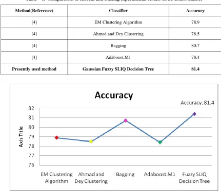
learning in Quest (SLIQ) decision tree (FS-DT) algorithm” in classifying breast cancer cases, which produced finest results over techniques used beforehand in categorizing Benign and malignant breast cancer instances on BI-RADS data. Coming to the UCI Repository datasets, various classifiers showed various accuracies. [3] Kamadi VSRP Varma et.al applied the Fuzzy SILQ Decision Tree method on diabetes disease and obtained better accuracy rate than the existing classifier techniques. Similarly when we applied the proposed model Fuzzy SLIQ Decision Tree method on BI-RADS dataset, we got better results than the existing classifier techniques. [4] Adaboost.M1 gave an accuracy of 78.4% , Ahmad and Dey Clustering technique gave an accuracy of 78.5%, EM Clustering Algorithm gave an accuracy of 78.9%, Bagging technique gave an accuracy 0f 80.7% and the proposed system Fuzzy Decision Tree gave an accuracy of 81.4% on BIRADS dataset, which is better than the existing systems. The results have been displayed in Table.2. The rest of the paper is organized as follows; Section II describes flow chart of proposed model and its description; Results were discussed in Section III. Conclusion and scope for further work was discussed in Section IV.

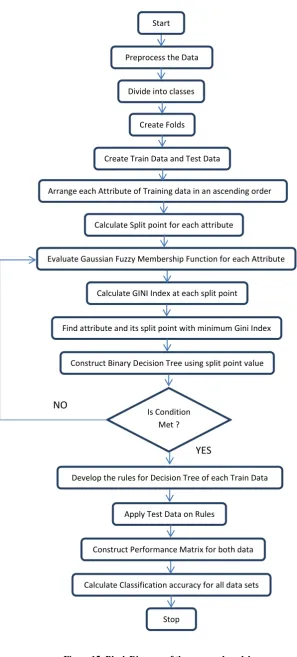
2.

DESCRIPTION OF PROPOSED

MODEL

2.1 Algorithm of the Proposed Model

1. Start

2. Preprocess the data

3. Divide the data into number of classes

4. Divide each class into three folds ( Three fold cross validation )

5. Construct the three folds into three training and testing data sets

6. Read the training data set

7. Arrange each attribute in ascending order

8. For each attribute arranged in an order calculate the split points

9. Identify the split points where class change occurred which have different attribute value

10. Exclude all the false split points

11. For each split point evaluate Gaussian membership function

12. Calculate Gini Index at each split point 13. Identify the attribute and split point which have

minimum Gini index

14. Using split point, construct a binary decision tree for training data with left and right child nodes 15. Repeat the process for each node from step-2 until

stopping criterion is met.

a. If all records fit into same class b. If all records have same attribute values c. If no more records were left

16. Formulate the rules for the obtained decision tree 17. Apply testing data on the rules

18. Construct the performance matrix for training and testing data

19. Calculate the classification accuracy, sensitivity and specificity for all train and test data sets

20. Stop

As previously discussed this dataset consists of six attributes in total. After necessary preprocessing done by filling all the missing data values with their mean values, we have classified all the 961 instances into two classes. The first class is classified as non-cancerous and the second class is classified as cancerous cases. From these two classes we extracted three folds using some technique. We may extend the folds according to our wish as folds3, folds5, folds10 and so on. Now from these folds we prepare a training dataset as well as testing dataset. Now read the training dataset and consider individual attribute and arrange them in ascending order. For each attribute arranged in ascending order calculate the split point. Whenever there was a change in class value and corresponding attribute value we consider it as a split point. For each split point calculate membership function.

2.2 Membership Function

A [6] membership function for a fuzzy set A on the universe of X is defined as µA:X → [0,1], where each element of X is charted to a value between 0 and 1. This value, called as membership value or degree of membership, measures the grade of membership of the element in X to the fuzzy set A. Membership functions allow us to graphically represent a fuzzy set. The x axis represents the universe of discourse, whereas the y axis represents the degrees of membership in the [0,1] interval. Below is a list of the membership functions

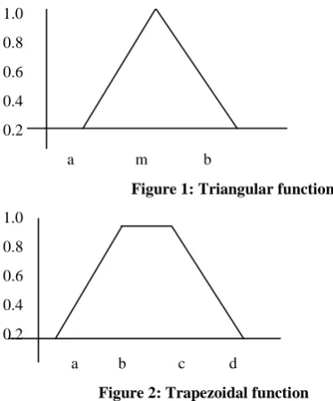
2.2.1 Triangular and Trapezoidal functions:

Triangular function is defined by a lower limit a, an upper limit b, and a value m, where a < m < b. 1.0

0.8 0.6 0.4 0.2

a m b Figure 1: Triangular function

1.0 0.8 0.6 0.4 0.2

a b c d Figure 2: Trapezoidal function

Whereas Trapezoidal function is defined by a lower limit a, an upper limit d, a lower support limit b, and an upper support limit c, where a < b < c < d.

2.2.2 Gaussian function:

Gaussian function is defined by a central value m and a standard deviation k > 0. The smaller k is, the narrower the “bell” is.

1.0 0.8 0.6

0.4 μA x = e−

(x−m )2

2k2 (1) 0.2

m

Figure 3 : Gaussian function

2.3 Gini Index

The Gini index is evaluated for each split point value for all the attributes. The split-measure Gini index is customized for evaluating the best split in the fuzzy decision tree algorithm. The formula is given as follows:

D xj = N

(v)

N(u)

v

v=1 1 −

N_{w k}(v) N(v)

2 C

k=1 where , (2) C represents the total number of classes;

V denotes the total number of partitions;

N(u) indicates the sum of the fuzzy membership values of the records in the dataset before split if Xj is chosen as the split point;

N(v) implies the sum of the fuzzy membership values of the records in the V th partition;

N(v)wkwk entails the sum of the product of the fuzzy membership values of the attribute and the fuzzy membership values of the corresponding records for class wk in the V th

2.4 Decision Tree

After calculating the gini Index, find the attribute and the corresponding split point which has the minimum gini index value. Now consider the minimum gini index attribute as the node and start constructing the decision tree with left and right child nodes using the split point value. Repeat the process for each node until the stopping criteria is met. That is,

i. If all records in the dataset belong to the same class ii. If all records have similar attribute value

iii. If no more samples are left in the dataset

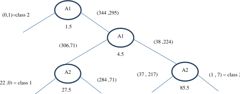
A Sample Decision tree for training dataset – 1 is shown in figure 16. Similarly decision tree is constructed for Train2 and Train3 datasets.

2.5 Develop Rules

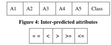
Rule condition is of the form “ Ai OP Vij ”; Where „Ai‟ represents the i-th inter-predicted attribute, „OP‟ represents the assessment operator {<, >, <=, >=, = =} and „Vij‟ denotes j-th value of the i-th attribute. The predicted attributes for the BI-RADS database is shown in figure 4. And the operators used for combining the attributes are shown in figure 5.

A1 A2 A3 A4 A5 Class

Figure 4: Inter-predicted attributes

= = < > >= <=

Figure 5: Operators for inter-predicted attribute values.

Sample rules for the above decision tree are i. If (A1) <=1.5 then class is 2

ii. Else if (A1) >1.5 and (A1)<=4.5 and (A2)<=27.5) then class is 1

iii. Else if (A1)>1.5 and (A2)>85.5 then class 2 else soon…

Like this the rules will be developed for the obtained decision tree for each training datasets. Since we considered a threefold cross validation of the BI-RADS dataset, we get three

decision trees for each training datasets 1,2,3 and hence corresponding rules for each decision tree will be developed. After developing rules for all the decision trees, apply the testing data on the obtained rules for each training dataset. Construct the Confusion matrix.

2.6 Confusion Matrix

A [8] confusion matrix, also known as a contingency table or

Figure 6: Confusion Matrix

an error matrix , is a specific table layout that allows visualization of the performance of an algorithm, typically a supervised learning (in unsupervised learning it is usually called a matching matrix). Each column of the matrix represents the instances in a predicted class, while each row represents the instances in an actual class. The name stems from the fact that it makes it easy to see if the system is confusing two classes (i.e. commonly mislabeling one as another).

Table-1: Formulas of accuracy, sensitivity and specificity

Measure Formula

Accuracy FN FP TN TP TN TP     Sensitivity FN TP TP  Specificity FP TN TN 

3.

RESULTS

We used BI-RADS data set with three fold cross validation for classification of benign and malignant cases. First training set is partitioned into 640 tuples of fold 2 and fold 3 values and first testing set is partitioned into 321 tuples of fold 1 values, in total 961 tuples which is a complete BI-RADS dataset. Similarly second training set with 641 tuples of fold1 and flod3 values and corresponding test set with 320tuples of fold two values out of 961 total tuples. And finally the third set with 641 tuples of fold1 and fold2 values and the corresponding testing set with 320 tuples of fold3 values. BI-RADS data set has missing values in each attribute. We replaced all the missing values of the corresponding attribute with the average of the attribute values. First the system is trained up with the training datasets and then it is tested with the testing datasets for all the three folds using the rules developed by the Gaussian fuzzy SLIQ decision tree algorithm. The specificity, sensitivity and the accuracy results for Training dataset – 1 with three testing data sets are presented in table 2.The average accuracy results for Training dataset – 2 with three testing data set are presented in table 3. The average accuracy results for Training dataset – 3 with three testing data set are presented in table 4. Finally we have to consider accuracy results of Train – 1(fold2, fold3) and Test – 1(fold1) values, Train – 2(fold1, fold3) and Test –

True Positive

False Negative

False Positive

True Negative

2(fold2) values and Train – 3 (fold1, fold2) and Test – 3(fold3) values which form complete BI-RADS Dataset for three fold cross validation. If we use any other combination one set of fold values will be missed in result calculation. The final Average classification accuracy of BI-RADS dataset using Gaussian Fuzzy SLIQ Decision Tree Algorithm using three fold cross validation is displayed in table 5. The comparison of the current results with already existing results of various methods on BI-RADS dataset is displayed in table 6 and the graphical representation of the comparison results are shown in figure 14.

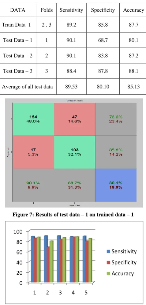
Table – 2: The specificity, sensitivity and the accuracy results for Training dataset – 1 with three testing datasets

DATA Folds Sensitivity Specificity Accuracy

Train Data 1 2 , 3 89.2 85.8 87.7

Test Data – 1 1 90.1 68.7 80.1

Test Data – 2 2 90.1 83.8 87.2

Test Data – 3 3 88.4 87.8 88.1

Average of all test data 89.53 80.10 85.13

Figure 7: Results of test data – 1 on trained data – 1

Figure 8: The specificity, sensitivity and the accuracy results for Training dataset – 1 with three testing datasets

along with the average of all test data result

Table – 3: The specificity, sensitivity and the accuracy results for Training dataset – 2 with three testing datasets

DATA Folds Sensitivity Specificity Accuracy Train Data 2 1 , 3 90.4 81.5 86.3

Test Data – 1 1 95.3 74.0 85.4

Test Data – 2 2 80.2 83.8 85.4

Test Data – 3 3 85.5 89.2 87.2

Average of all test data 87.0 82.3 86.0

Figure 9: Results of test data – 2 on trained data – 2

Figure –10: The specificity, sensitivity and the accuracy results for Training dataset – 2 with three testing datasets

along with the average of all test data result

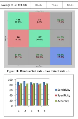
Table – 4: The specificity, sensitivity and the accuracy results for Training dataset – 3 with three testing datasets

DATA Folds Sensitivity Specificity Accuracy

Train Data 3 1 , 2 89.5 75.5 83.0

Test Data – 1 1 91.8 72.0 82.6

Test Data – 2 2 87.2 79.1 83.4

Test Data – 3 3 84.9 79.1 82.2

0 20 40 60 80 100

1 2 3 4 5

Sensitivity

Specificity

Accuracy

0 20 40 60 80 100

1 2 3 4 5

Sensitivity

Specificity

Average of all test data 87.96 76.73 82.73

Figure 11: Results of test data – 3 on trained data – 3

Figure 12: The specificity, sensitivity and the accuracy results for Training dataset – 1 with three testing datasets

along with the average of all test data result

Table – 5: The specificity, sensitivity, accuracy and average results for all training and testing BI-RADS

datasets

DATA Folds Sensitivity Specificity Accuracy Train – 1,

Test – 1

(2 , 3),

( 1) 90.1 68.7 80.1

Train – 2, Test – 2

(1 , 3),

( 2) 80.2 83.8 81.9

Train – 3, Test – 3

(1 , 2), ( 3)

84.9 79.1 82.2

Average of complete

dataset 85.06 77.2 81.4

Figure 13: The specificity, sensitivity and the accuracy results for Training dataset – 1 with three testing datasets

along with the average of all test data result

4.

CONCLUSION

From the results obtained using Gaussian Fuzzy SLIQ Decision Tree Algorithm for various rules when applied on all training and testing BI-RADS datasets, we achieved better classification accuracy rate of 81.4 which is better than existing techniques where their results ranged between 78.4 and 80.7 which are shown in table.6. Also as a future work we may apply this Gaussian Fuzzy SLIQ Decision Tree Algorithm on each field and their sub fields and analyzed the importance of each field and their sub fields based on the classification accuracy obtained. For example if we consider the Mass shape field, we can find which of the sub fields like round, oval, lobular and irregular plays prominent role in acquiring better classification accuracy. Similarly the prominence of other fields and their sub fields like Mass-Margin: circumscribed, microlobulated, obscured, ill-defined and speculated; Mass-Density: high, iso, low and fat-containing can also be examined in classification accuracy and identify the vital and non-vital fields and their sub fields in dataset classification. Also, we may try to improve the classification accuracy by bringing up a New or a hybrid model which classifies the BI-RADS data more accurately then the existing methods. We may also try this method in other cancer datasets and find out the classification accuracy.

5.

ACKNOWLEDGEMENTS

Our sincere thanks to the UCI Machine Learning Repository for providing the BI-RADS breast cancer dataset. My special thanks to my head of the department, Computer Science and Engineering, Prof P V Nageswar Rao and the management of GITAM UNIVERSITY, VISAKHAPATNAM, INDIA, for providing me the necessary software and resources in carrying out the research work. My sincere thanks to my wife S.Jaya Kalyani for helping me in all ways in carrying out my research work smoothly.

6.

REFERENCES

[1] R.A. Smith, "Epidemiology of breast cancer in a categorical course in physics,” Technical Aspects of Breast Imaging, 2nd ed., RSNA publication, Oak Book, II, pp.21, 1993

[2] M. Mehta, R. Agrawal, and J. Rissanen, “SLIQ: A fast scalable classifier for data mining,” in Proc. Extending Database Technol.

[3] Kamadi V S R P Varma, Dr. Allam Apparao, Dr.T.Sitamahalakshmi, Dr. P.V .Nageswar Rao, K.Narasimharao, NCETCS‟14 (pages289-295) A

0 20 40 60 80 100

1 2 3 4 5

Sensitivity

Specificity

Accuracy

0 20 40 60 80 100

1 2 3 4 5 6 7

Sensitivity

Specificity

Computational Intelligence technique for effective diagnosis of diabetes disease using Genetic Algorithm.

[4] SM Halawani, M Alhaddad and A Ahmad (2012).JSIR, Vol 71,pp594-600. A study of digital mammograms by using clustering algorithms.

[5] Archive.Ics.Uci.Edu/Ml/Machine-Learning-databases /mammographic-masses/mammographic _masses.data

[6] www.dma.fi.upm.es/java/fuzzy/fuzzyinf/funperten.htm [7] Hameed IA, Gaussian Membership functions for

improving the reliability and robustness of students evolution system. ExpSystAppl 2011.

[8] Sofia Visa, Brian Ramsay,Anca Ralescu,Esther vander Knaap, Confusion Matrix- based Feature Selection http://ceur-ws.org/Vol-710/paper37.pdf

Table – 6: Comparisons of current and existing experimental results on BI-RADS dataset

Method(Reference) Classifier Accuracy

[4] EM Clustering Algorithm 78.9

[4] Ahmad and Dey Clustering 78.5

[4] Bagging 80.7

[4] Adaboost.M1 78.4

Presently used method Gaussian Fuzzy SLIQ Decision Tree 81.4

Figure 15: Block Diagram of the proposed model

NO

YES

Divide into classes

Create Folds

Create Train Data and Test Data

Arrange each Attribute of Training data in an ascending order

Calculate Split point for each attribute

Evaluate Gaussian Fuzzy Membership Function for each Attribute

Find attribute and its split point with minimum Gini Index

Is Condition Met ?

Develop the rules for Decision Tree of each Train Data

Calculate Classification accuracy for all data sets Calculate GINI Index at each split point

Construct Binary Decision Tree using split point value

Apply Test Data on Rules

Construct Performance Matrix for both data

Figure 16: Sample Decision tree for BI-RADS Train1 Dataset of 640 records A1

A1 (0,1)=class 2

1.5

(344 ,295)

(306,71)

4.5

(38 ,224)

A2 (22 ,0) = class 1

27.5

(284 ,71)

A2 (37 , 217)

85.5