Some problems in nonlinear elasticity

Thesis by

Michael Alan Kosecof:f

In Partial Fulfillment of the Requiren~ents for the Degree of

Doctor of Philosophy

California Institute of Technology Pas adena, California

1975

-i~.

-ACKNOWLEDGEMENTS

I wish to thank Professor Herb~rt B. Keller for suggesting the problems and for his valuable guidance in their pursuance. I an-:. also indebted to Professors DonaldS. Cohen, Edward L. Reiss, Charles D. Babcock, and Paco A. La~erstrom; discussion~:; with each of them have proven useful at some point in this work. Mrs. Karen Cheetham and Mrs. Virginia Conner undertook the task of typing this symbol-ridden manuscript in a rather brief period of time, and I truly appreciate their labors. Finally, to my wife, Jackie, I owe more than can fit into this short space.

ABSTRACT

Two separate problems are discus sed: axisymrnetric eqt::.ili -brium configurations of a circu.la:c n1err1b!"ane under pres sure and

subject to thrust along its edge, and the buckling of a circular cylindrical shell,

An ordinary differential eqt.;.ation governing the circular men1-brane is imbedded in a family of n-dimensional nonlinear equations. Phase plane methods are used to examine the nurnber of solutions corresponding to a parameter which generalizes the thrust, as well as other parameters determining the shape of the nonlinearity and the undeformed shape of the membrane, It is found that in any nurnber of dimensions there exists a value of the· generalized thrust for which a countable jnfinity of solutions exist if son1.e of the re1naining parameters are made sufficiently large. Criteria describing the number of

solutions in other cases are also given.

Donnell-type equations are used to model a circular cylindrical shell, The s.tatic problem of bifurcation of buckled modes from

Poisson expansion is analyzed using an iteration scheme and pertubation methods. Analysis shows that although buckling loads are usually

simple eigenvalues, they may have arbitrarily large but finite multi-plicity when the ratio of the shell's length and circumference is rational. A numerical study of the critical buckling load for simple eigenvalues indicates that the number of waves along the axis of the deformed shell is roughly proportional to the length of the shell, suggesting the possi-bility of a "characteristic length. " Further numerical work indicates

-)·

v-may increase or decrease. It is shown that either a sheet of solutions or two distinct branches bifurcate from a double eigenvalue. Further-more, a shell may be subject to a uniform torque, even though one is not prescribed at the ends of the shell, th1:ough the interaction of two modes with the same number of circumferential waves. Finally, !nultiple time scale techniques are used to study the dynamic buckling of a rectangular plate as well as a circular cylindrical shell; transition to a new steady state amplitude determined by the nonlinearity is

Chapter 0 l 2 3 4

TABLE OF CONTENTS Title

Introduction

Part I: Circular Men1.branes Initially flat mernbrane s

Preliminaries The case n

>

2 The case n

=

2 The case n

=

l Initially curved membranes

Preliminaries

Small amplitude pertubations, 0 <

lA

I

<< 1

Large amplitude pertubations,

.

lA

I>>

l

Infinite multiplicities

Part II: Circular Cylindrical Shells The static problem

Preliminaries

Decomposition of the Airy stress function

Symmetric solutions

Poisson expansion and bifurcation Multiplicity of the eigenvalues The buckling mode

Bifurcation for simple eigenvalues Bifurcation for double eigenvalues The dynamic problem

Premliminarie s

The rectangular plate

The circular cylindrical shell

Chapter

A B

c

-vi-TABLE OF CONTENTS (cont1_d) Title

Appendices

Derivation of shell equations Some calculations for Chapter 4 Notes on the membrane equations

References

INTRODUCTION

This study is concerned with two separate problems. The first is motivated by equations which n-wdel the behavior of a circular

rnern-brane. The resulting equation is imbedded in a class of equations, anu

the existence of multiple solutions is analyzed fo::.- this class. The

second problem is to study the static and dynamic buckling of a circular

cylindrical shell under axial loading.

F'or the first problem, we are concerned with studying the

possibility of multiple equilibriu1n configurations of a circular shallow

elastic n1embrane whose surface is subject to an axisymmetric

pres-sure. A radial thrust is specified along the membrane 1 _{s edge, and tJ::.e}

edge is restrained from deforming normal to its midplane. Only

axi-symmetric deformations of the membrane are considered.

In chapter 1 we study the case of an initially flat membrane

under a variable pressure. The situation of a flat membrane under

constant pressure has been studied by A, Callegari, E. Reiss, and

H. Keller [2]. In chapter 2 we consider a membrane which is not

initially flat and is subjected to a variable pressure,

The reader is referred to the references [1, 2] for a derivation

of the membrane theory. Notes on the final formulation of the problem

are given in Appendix C. The resulting equation is

(C. 6)

The boundary conditions are

du

-2-u(l) = 0 (C. ?b}

When G{r) and ~(r) are of the form to be prescribed in chapters

1 and 2, it is found that equation (C. 6) can be transformed into a

second o1·der autonomous system which is amenable to phase pla:ne

analysis. This method was first used by Gel' fand [ 4] to study solution multiplicity in certain problerns arising in the theory of :::hemical

reactors, viz.

1 d n-1 du u

(

)

+

A e

n-1

dr r dr

r

du __

0 at r dr

u(l) = 0

=

0 n ·- 1, 2, 3

=

0

He found that there exists a value A . _,,._ _.

>

0 such that there are (a) no solutions when A > A>:, (n = 1, 2, 3)

(b) one solution when A

=

A._ _>,. (n

=

1, 2, 3) (c) two solutions when 0

<

A < A,:< (n = l, 2)

l

j

(0. l)

(d) a countable infinity of solutions when A

= A"'

=

2 and n -· 3 (e) a finite but large number of solutions when n

=

3 and

I

A - A"'

I

is small.

A. Callegari, E. Reiss, and H. Keller [2] applied this method to study an initially flat circular membrane under constant pressure,

modeled by

=

0

Here the differential operator is a Laplacian in four dimensions (n

=

4).

Joseph and Lundgren [8] studied (O.l) and

l d l n-1 du)

+ '('

)l-13 ₀

-n-1 dr ,r dr 1\. i -au = (0. 2)

r

for arbitrary positive integers n and for ~

>

1, a

>

0. For (0. l) they

found that (a) and (b) hold for n;;:: 1, that (d) and {e) hold for 2 < n < 10

with A

=

n(n-2 ), and that for n :2: l 0 there exists one soluEon

fo:::-co

A< 2(n-2). For (0. 2) they found (a) and (b) hold for n :2: 1, (d) and (e)

hold when n-2 < f(l3 ), and for n-2 :2: f(l3) there is only one solution in

0 < A < A,... _..,, Here

f(P.)

=

4~:..!J

+

4

'!FT"

t-'

13'

y 13"

(Note: [8] also includes a similar study for

a<

0 and 13 < 1).

In chapters 1 and 2 of this study we find that equation (C. 6 ),

for appropriate functions G and

rp,

is of the type

_I ~ ( n-1 du) + Al3 !.l(l )1-13 _ A.A 2+(1J.+2)/!3

n-ldr r dr r -au - ~r (0. 3)

r

with 13

>

1 and a

f.

0. We investigate solutions of (0. 3) for all real

A,

thereby generalizing the results of [8]. Of particular interest is the

result that for a > 0 there exist values ~L':' (for n :2: 1) and A

₀

(for n ~ 3)

such that if 1-l

>

!.l':' or A

>

A0 , then the situation may be described by

(a), (b), (d), and {e) with appropriate A

00• (The cases of A large and

n

=

l, 2 are not investigated here.) From this we see that the possi

-bility of an infinity of solutions persists in all dimension~. We

summarize our results below.

For A

=

0 there exist A,:, and !.l':' such that, for n ~ 1, there are

{a) no solutions for aA!3

(b) one solution for a\.13

13

> a:\ ... > 0

.

.

·-·

'%:'-(c) finitely many solutions for 0 < aAP <

D.'A

,

_,,,

~

if f-L s: fl.,:,

(d) a countable infinity of solutions when A

=

;,.::o

if f-t

>

fl.,:,

(e) a finite but large number of solutions if

I)

,

-

A eo

l

f-

0 is srnall

Here fl.':' is such that .P(fl->!<+ 2)

=

0, where

(1. 23}

For A /: 0 we restrict !3 to integral values and take n > 2. When !A I

<<

1 the situation is the same as for A

=

0, except that fl.':' depends on

A. For !A

l

sufficiently large we find

(a}

!3

odd, A> 0,

a> 0: For

A> 0 there exist A _eo and A_,_ _{.. ~ ..} as above.

For A.

<

0 either there exists one solution for all A. or

A.; exists such that no solutions exist for A. < A::;~ and

finitely many exist for A.,;

<

A. < 0.

(b)

!3

odd, A

<

0, a

>

0: For A. > 0, A..,_ exists but there is no A.

~ ro

and hence there are only finitely many solutions. For

A.

<

0, there exists one solution for all A..

(c)

!3

even, A >. 0, a > 0: A::;<' A.'Xl, and A.,; as above all exist. (d)

!3

even, A > 0, a

<

0: For A. > 0 either there exists one

solution for all A. or A._.. .~ _,~ exists but A. _CCI does not. For A. < 0

there exists one solution for all A..

The cases omitted may be found by transforming a -+ -a, A. -+ -A. for

!3

odd and A -+ -A, A. -+ -A. for

!3

even.

For the second problem, we are concerned with studying the

L""l chapter 3 we consider the static problem. The classical solution

known .as Poisson expansion is introduced, and the problen1 of the bifurcation of equilibrium states from this solution is fornmlatecl. We analyze the :multiplicity (i.e., the number of independent

eigen-functions) o£ eigenvalues or buckling loads and find that although they are typically simple, an arbitrarily large albeit finite multiplicity j s

possible when the ratio of the shell's circumference and length is rational. A numerical study is made of the mode corresponding to the

critical buckling load, and it is found that the number of waves along the axis of the shell is roughly proportional to the length of the shell,

suggesting the possibility of a "characteristic length" over which buckling occurs. An iteration scheme developed by H. Keller and

W. Langford [13] is utilized

to

calculate the initial post-buckling curve for simple eigenvalues. We find that the load may increase or decrease, but regardless, the load-deflection curve is usually very steep. A

pertubation scheme is used to study the number of bifurcating branches when the buckling load is a double eigenvalue. Several possibilities occur: there may exist a one or two-parameter "sheet" of solutions, or else there exist precisely two branches of solutions. A final calcu-lation shows that, through the interaction of two modes with the sarne number of circumferential waves, the shell may be subjected to non-vanishing uniform torque even though no torque is prescribed at the ends of the shell.

Chapter 4 treats the dynamic problem when the load is such that Poisson. expansion is unstable. The load is taken to be a "sn"lall

-6-multiple time scales is '..ltilized. This rnethod was first used by

B. Matkowsky[l4]. We first apply it to the dynamic buckling of a

rectangular plate, and the results are compared to those of a study by

Reiss and Matkowsky[l5] of the buckling of rods. The equation

governing the amplitude of the unstable mode is found to be a second

order autonomous equation in the absence of damping. However, the

equilibrium points depend on the initial conditions, which contradicts

the fact that equilibrium configurations satisfy the time -independent

steady state equations. When damping is present, the terms depending

on the initial conditions vanish exponentially, and bounded solutions

are shown to be asymptotic to the critical points of a reduced

auton-omous system. A similar discussion applies to the problem of a.

circular cylindrical shell. Qualitatively the two problems differ in

that the reduced system for a plate is two dimensional, but that of a

cyLindrical shell is four dimensional. Also the plate has two physically

distinct stable equilibrium configurations, but the cylindri~al shell has

only one. (For both problems we assume that the critical eigenvalue

CHAPTER 1: INITIALLY FLAT MElviBR.<\NES

In this chapter we will analyze the number of equilibrium configurations of an initially flat n1.embrane subject to a pressure

distribution of the forrn

for c ~ 0. Substituting this into the formulae given in equations (C. l) results in

G(r) p

=

r

=

j.L

+

3 2

where we have set f-l = 2c. A flat tnembrane 1s descr1bed by ~(r) - 0; hence equation (C. 6) becomes

d2 u 3 du

+

,

3 ri-L

+

r dr A -- 0

dr2 (l-u)2

subject to boundary conditions (C. 7 ). d2 3 d

Recognizing -d 2

+-

-d as a spherically syrnn1.etric Laplacian r r r

in four dimensions motivates the following simple generalization of the

membrane problem:

( l. l)

l' _{lmr ...}

o

I

.!.

_r du

I

<

cx:-dr (l. 2)

u(l) = 0 (l. 3)

-8-the nonlinearity will play a strategic role in certain of -8-the argu.ments

to follow.

We seek a solution u E: C2 (0, 1 ), so equation (1. l) implies that

1-au(r)

-J

0 for 0 < r < 1. u(l) = 0 and contim1ity then imply that I -au > 0

in (0, l

J.

We extend this a.nd require

l-au(r) > 0 (l. 4)

Elementary considerations using t.he theor·y of l,ie ]ead to the following

change of variables:

where

x == log r

v(x)

=

(l -cm)r Y

y

=

-(~+2)/!3

(l. 5)

{1. 6)

{ l. 7)

Note that y

<

0. These new variables transform. equation (1.1) into

the equivalent a'~tonornous equation

(Zy +2 -·n):

+

y (Y + 2 -n)v - a\!3 vl-!3

=

0

or

dv !3 1 -!3

(y +e) dx

+

y 8v-aA. v :: 0 (1. 8)

where we have defined 8

=

y- (n-2) ( 1. 9 j

Boundary conditions (1. 2) and (1. 3) become respectively

1. _{1mx_.} -a:> e -(y+2)x ·

I

dv dx - y v

I

<<X (1. 10)

and

v = l at x = 0 (1.11)

Remark also that condition (1. 4) implies

v -.

+

a:> as x -t -a:> (1. 12)

-9-Although it is possible to study equation (l. 8) in the phase plane

directly, one last change of variables proves to greatly sim.plify the

analysis. Set

y(x)

=

aJ..f-lv -(j

1 dv

z(x)

= -:;;

dx

We find that equation (1. 8) is equivalent to the system

(!.13)

(l. 14)

.

y

=

-f>yz

=

f(y, z) (l. 15a)

z

=

y- {.z-y)(z-8)

=

g(y, z) (1. 15h)

where differentiation with respect to x is indicated hy a dot. The

boundary conditions become

-(v+2)x

I

~--l;'P..

lim e ' ( z -·y) y ~--' x-+ -co .

<

c:c

y(O)

=

a! .. f>

Furthern~ore, (1.12), {l. l3) and the hypothesis

p

> l irnply

y-+0 as x -+ -ex

In making the transformation (1. 13) we have tacitly assum~d that

(1. i6)

(1.17)

(1.18)

A.

f.

0. When A.= 0 it is easily verified that equations (1. 1), (1. 2) and

(1. 3) have the unique solution

u(r) == 0

for n

>

0. In the remainder of the chapter a/...f>

/=

0 will be presumed.

Depending on the dimension, three cases arise in the phase

plane analysis, namely: n

>

2, n

=

2 and n

=

1.

The case n > 2

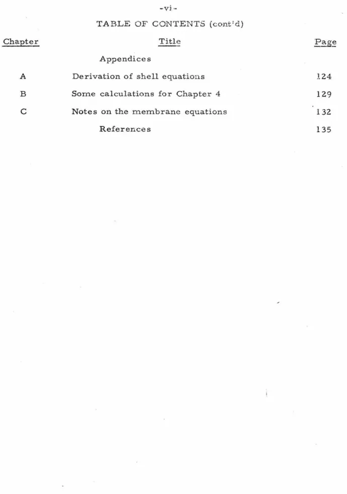
Frotn (1. 9) we see that 8 < y < 0. System (1. 15) has three

-10-P2:

y =

o,

z

= e

P3 : y

=

y8, z

=

0

In figure 2 we indicate the field of tangent vectors corresponding to

system (1. 15), including the locus

r

where~= g(y, z)

=

0. Note that

y == 0, ;.; ~ -(z-y)(z-'8) provides three exact solutions wnose trajectories

completely cover the z axis; consequently no trajectory can cross the

z axis.

Next consicier the local behavior about each critical point. 'Ne

readily compute f _y = -[3z, f = -{3y, g = 1, g

=

-2z + y + 8 and so the

z y z

equation for the characteristic exponent 1- at the critical point (y_{0 ,} z0 ) j_s

-{3zo

-.e

=

0 (1.19)

l -2.zo +y+8 -J',

For P1, y0

=

0, zo

=

y and (1.'19) becomes

--{3y-£ 0

=

0

1

8-v-£

which has roots £ _{= ..21}

=

-{3y and£

=

£2

= 8-y

Now -{3y

=

!J-+2 > 0 and

8 -Y = -(n-2)

<

0 for n

>

2. Consequently P1 is always a saddle point.

For P2 , y0

=

0, z0

=

8 and the roots are £1 = -{38 and £2

=

y-8.

{3

>

1 and 8 < 0 mean £,₁

>

0. y-6

=

n-2

>

0 for n

>

2 mean £2

>

0.

Consequently, P₂ is an unstable node. Furthermore,

p

> 1 and n

>

2

imply that P2 is an in~proper node, for recalling the definitions of y

and ewe find

£1 - -{38

=

-{3y + p(n-2)

=

(!J-+2)+ p(n-2)

>

n-2

=

y -9

=

£₂

To de scribe the behavior near P2 in more detail, set

z

_ r

Figure 2 The field of tangent vectors for n > 2

\)

.. ~.

2-vre obtain the linea.rized form of equations (1. 15)

which has solutions

{; -(3 8x

.., = ae

C

=

b e(n-2)x a. _e -f36x

[38

+

n-2

l

j

(1. 20)

Since P₂ is an unstable node, trajectories approach P₂ for

x -+

-=.

This, and the relation -[3 S > n-2 > 0 imply that trajectories

are tangent to the

C

\or z} axis unless b = 0, in which case there exist

two trajectories tangent to the line

£

+ ((36

+

n-2)s = 0.

For P3 , y0 = y9, z0

=

0 and the characteristic equation is

which has roots

(1.21)

Now 4(3y8 = -4(f.L+2)9

>

0 so that the real parts of

.t

1 and

.t

2 always have

the same sign; consequently P3 is always an attractor (i.e., a spiral

point or a node). Furthermore, y+9

<

0 so that P₃ is a stable attractor.

Consider first when P3 is a spiral point, i.e.,

This relation is equivalent to the following inequality in t,erms of the

original parameters [3, f.L and n:

( 1. 22)

where

Figure 3 shc·ws the qualitative behavior of <f>(\i} for

f3

>I,

n > 2. In the

region

v

> 0, <ii decreases n1onotonically, so for given

f3

and n, we have

a spiral for all i-l ~ fl.':' i£ and only i£ i.P(!-l-':'+2) < 0. In particular, P3 is a

spiral point for all fl. :<: 0 if i.P(2)

<

0, and this can be shown to be

equivalent to

f3

2

(n-2)(n-10} + 8[3(n-4) +16 < 0 (1. 24)

For the membrane problem origin.ally proposec4 n

=

4 and

f3

=

3; it is

a simple matter to verify that (1. 24) is indeed satisfied for these values

of the parameters. lvfore generally, for given values of n

>

2 and

p

> 1

there exists a value fl.':' such that for all fl. >fl.':', P3 is a spiral point.

Next we consider the structure of the phase plane near P3 ·when

it is a node. (It will turn out that the local structure about P3 critically

determines the number of equilibrium· solutions of the membrane

proble1n.) Set y

=

ye

+

L

z

=

C;

the linearized form of equations {1. 15)

is now

(~)

=

(~

-f3y8) _Y

+

e

(~)

c

Eigenfunctions

(~)

satisfy

-f3y8 )

(Cl) _

(0)

y+G-~ c2 0

or c₁

=

[~-(y+8)]c

2

• Note from equations (I. 21) that

~ -(y+8) = -~2

The linearized theory in the neighborhood of P3 thus provides the

-14-(~)

for some constants a, b for a given trajectory. Since

.

e

₂

<

.t1

<

0, we

can conclude fron'l this that in a neighborh.ood of P3 all trajectories are

tangent to the line y - y 8

+ /.,

2 z

=

0, except for one pair of t raj e cto rie s

which is tangent to the line y- y8

+

1.,₁ z

=

0.

In the special case that /.,2 = 1.,1

<

0, there is only one

eigen--vector, and the general theory for critical points shows that P3 is

again an improper node with all trajectories tangent to the same line.

In figure 4 we summarize the above results about the behavior

of trajectories in a neighborhood of each of the finite critical points.

Some reference to figure 2 may also be helpful. We note in passing

that the tangent line to r at P3 is y - y8 + (Y+8 )z = 0. A justific3.tion

that the linearized theory does in fact accurately de scribe the behavior

of the solutions of the full nonlinear equations in neighborhoods oi each

of the critical points can be found in a standard reference, such as

Coddington and Levinson [3].

By combining the results of figures 2, 4a, and 4b we can

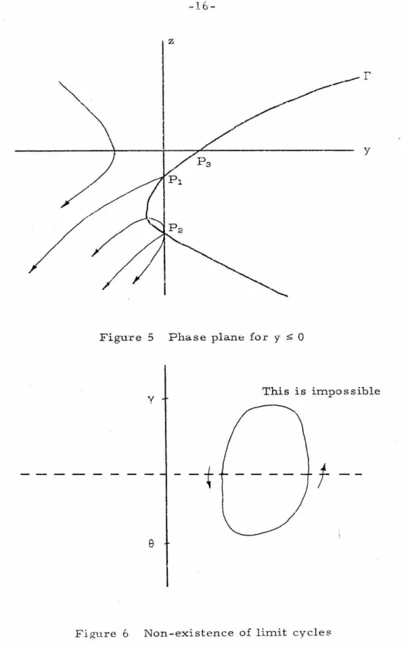
ascertain that the phase plane for y ~ 0 has the qualitative form of

figure 5, regardless of the behavior at P3 • vVe now concentrate on

completing the phase plane for y > 0. First we show that no limit cycles

exist. Introduce T] = log y and compute

ri

=

yjy

=

-(3z

=

F(n, z) }

(1. 25)

z

= y - ( z -y )( z - 8 ) = e Tl - ( z -y )( z -8 )

=

G( T) z )

z

(a) near P1

~r

/

(b) near P 2

"

\

(c) near P3 , spiral case

(d) near P3 , node with distinct eigenvalues

(e) near P3 , node with a double eigenvalue

-16-z

T '

.---

_..-l

y

/

/

/

Figure 5 Phase plane for y s: 0

y This is impossible

--t

f

--e

closed curve, say C, inclosing an area S. Vfe calculate, integrating

over one period in x:

0

=

r

(·n.~-;-n)dx ==

r

(~dz-~dTi}

.JC ' "C 'I •

=

J

8 'Y('!l. z) • (F, G)dnclz

=

J

(-2z+y+8)dT)dz

s

=

J

(Fdz -GdTJ)

c

(using Green1 _{s theorem)}

Consequently the lim.it cycle -:annat lie wholly above nor wholly below the line z

=

-t{y+8). (This is true in either phase plane, since T) is

merely a rescaling of the y axis.) However frotn either equation (1. 15) or figure 2 we conclude that

z

> 0 along the half-line y > 0, z

=

-t{y+8). This means that a trajectory can only cross this line in one sense (Cf. figure 6 ). It follows that no limit cycles exist.

Now consider the (unique) trajectory eminating from the saddle point P1 into the region y > 0. From the vector fielci we see that

y

>

0,

z

> 0 initially. Now either this trajectory intersects they axis in some

finite x, or else z < z0 s: 0 for all x, in which case z -+ z0 as x 4 +a:>.

But then we must also have ~ -+ 0 and y -+ +a:>. This is inconsistent with

.

z

=

y- (z -y)(z -8 ), so in fact this trajectory must inter sect the y axis at a finite point (necessarily to the right of the spiral point P3 ). From

the vector field (cf. figure 2) we can see that the trajectory then move s upward to the left, intersects

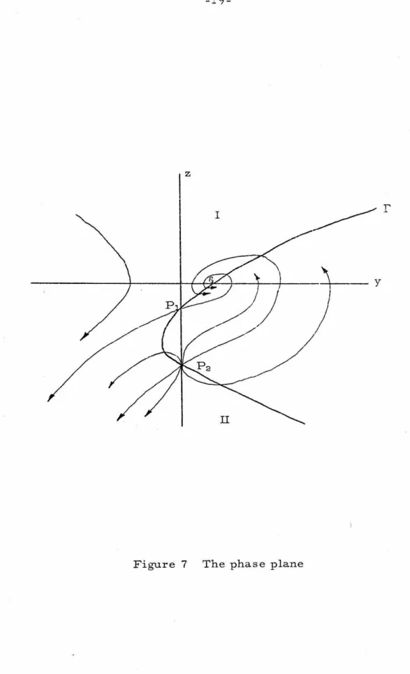
r

in the region 0 < z, continues downward to the left, intersects they axis in 0 < y < y8, and then continues down-ward to the right, intersecting I' in the region y < z < 0. Finally, the trajectory again moves upward to the right. We can now argue that the trajectory is bounded and, in the absence of limit cycles, necessarily

-18-If we take any point on

r

in the region y

>

0, z

<

8 a:::td follow the

trajectory through such a point as x -+

+Q,

exactly analogous ar~-un1.ents

apply. If we follow such a trajectory for x -+ -"', the vector field force3

it directly into the unstable node P2 • Thi::; discussion and the results

illustrated in figures 2 and 4 permit us to construct the phase plane

illustrated in figure 7 when P3 is the spiral point. Vlhen P3 is a node,

the plane remains qualitatively the same except in the neighborhood of

P3 , where trajectories either tend directly into the critical point or

spiral about it at most a finite number of times before tending into it.

Two possible families of trajectories tnay exist which have not

yet been discussed, their locations are indicated in figure 7 by region I

and region II. First we consider a point in region I. Necessarily as

x-+

+o.l

the trajectory through such a point tends to P3 • We have not

argued, however, that such a trajectory intersects the curve

r

(in the

region y > 0, z > 0) as x -+ -:co. If this does not occur, then y -+ -f-c:> and

z -+

+cr

as x -+

-co

Similarly, the trajectory through a point in region II

must tend to P2 as x -+ -co. vVe have not argued that such a trajectory

intersects

r

(in the region y > 0, z < 8) as x -+

+<X).

Should this not

occur, then y -+ +o:> and z -+ -co as x -+ +o:>. Fortunately, it will turn out

that these two possibilities are irrelevant to the boundary value problem

posed, and so further investigation is unnecessary.

We now search for trajectories in the full plane satisfying

boundary conditions (1. 16) and (1. 17), as well as the derived condition

(1.18). Consider first (1.18), viz. y(-o:>)

=

0. This eliminates all

trajectories except the two eminating from the saddle point P1 and

-19-y

-20-elin:tinates the possit?le trajecto2.·ies in region I mentioned above.

Consider trajectories tending to P2 as x--. -c:c. Along thern

z - y __. 8 - y

f

0, so rneeting boundary condition (1. 16) is equivalent to

-x(y+2)1 ~-l/[3

satisfying e y. · <"" as x __. -CXl. We derived in equation

(1. 20) the asymptotic relaticn y = ;'"""ae-f3Gx near P2 • The trajectories

satisfying a = 0 locally are, in fact, segments of the z axis withy= 0;

hence they cannot satisfy (1.17). Near P₂ boundary condition (1.16)

thus reduces to

-(y+2)':( -R8x)-l/P -(y+2)x+8x

e e ~""'

=

e

=

e -(y+2)x + (y-n+2)x = e -nx < ::::> as x __. -c::>

But this is not possible for n > 2, so that no trajectory tending to P₂

as x--. -c:c can satisfy (1. 16). In particular, this also eliminates the

possible trajectories in region II described above.

Our only hope for a solution, then, lies with the two trajectories

emanating from the saddle point P1 • With y =

£,

z = y

+

C

the

linear-ized equations for (~,

0

are

~ = -r:>Y s = <!J.+2)s

C =

s

+

(8-y)C =

£

-(n-2)C

with solutions

s

= ae(!J.+Z)x = ae-f3yx

( =be -(n-2 )x+ ~ e (!J.+2)x

- !J.+n

In the parameter domain n > 2 trajectories tending to

£

=

(

=

0 as

x --. -oo must have b

=

0. Thus as x --. -oo

and

-(y+2)x 1 ,-1/13 1 I -(y+2)x yx (fJ.+2)x fJ.X <

e y z-y ~ e e e

=

e co,

as x-+ -oo for fJ. ~ 0. Thus these two trajectories do indeed satisfy the boundary condition at x

=

-oo (corre spending to r

=

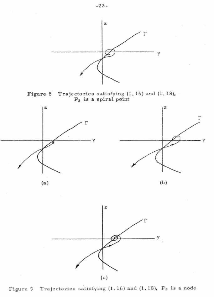
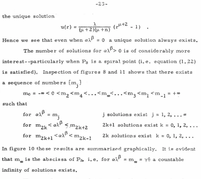
0),

In figure 8 we graph these two trajectories when P₃ 1s a spiral point. In figures 9 a, b, and c, we graph some typical examples when P3 is a node. In these latter cases the trajectory in the right half-plane may tend directly into P3 or may spiral about (at rnost) a finite number of times before tending into P3 • The analysis presented here is insufficient to determine precisely how 1nany times P₃ is encircled in the case of a node.

The remaining boundary conditio~ (1. 17), is trivial to satisfy; it merely requires that the solution trajectory intersect the line y

=

a1-J

3 when x

=

0. If a trajectory intersects the line y

=

a;\!3,

then the trans-lation invariance of the autGnomous system ( l. 15) implies that a

solution exists for which x

=

0 at the point of intersection.

The question of the number of solutions to equation (l. 1) with boundary conditions (1. 2) and (1. 3) is thus reduced to counting the number of intersections of the trajectories emanating from P1 with the line y = a;\!3 (each distinct point of intersection corresponds to a different transfonnation back to the independent variable 0 ::;; r ::;; l and hence a distinct solution).

Regardless of whether P3 is a spiral point or a node, precisely

one solution exists for every value of aA.f3 < 0. We noted earlier in the chapter that 'Nhen A.

=

0 the unique solution u(r)

=

0 exists. It is

-22

-z

y

Figure 8 Trajectories satisfying (1. 16) and (1. 18),

Ps is a spiral point

z z

I'

r

/ /

y y

//

/

/

(a) (b)

z

(c)

u(r)

=

A

(rf-

~+

2

-

l) ((!

+

2 )(}J.

+

n)

Hence we see that even when a\!3

=

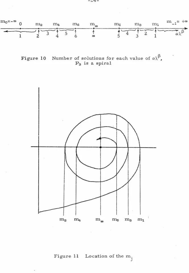
0 a unique solution always exists.

The number of solutions for a\!3> 0 is of considerably more interest--particularly when P3 is a spiral point (i.e. equation (l. ~2)

is satisfied). Inspection of fig..1re s 8 and ll shows that there exists

a sequence of numbers [ 1n.} J

rna

=

-co

<

0

<

:n ₂ < rn ₄ < ••• < m co< •••

<

n1.

3 < m

t

< 1n _1

=

+

co such that

for j solutions exist j = l, 2, ~

for 2k+l solutions exist k = 0, l~ 2,

for Zk solutions exist k

=

0, 1, 2, . •.

In figure 10 these results are su1nmariz~o graphically. It 1.s evid~nt

that rnco is the abscissa of P3 , i.e. for a\!3

=

m₀₀

=

y6 a countable

infinity of solutions exists.

We remark in passing that it was found earlier that for the

flat membrane P3 is a spiral point for all values of f.l· Consequently,

figure 10 depicts the distribution of equilibrium configurations ior

various edge thrusts and pres sure distributions.

When P₃ is a node the situation for aA.P> 0 is son1ewhat less

dramatic and, unfortunately, more vague. As can be seen from

figures 9a, b, and c, the separatrix connecting P1 and P₃ can tend

directly into P3 without any spiral behavior, or it can spiral a finite

number of times before tending into P3 • Consequently, a similar

sequence of m . can be constructed, with the difference that only a

J .

finite number of 111. exist and the nun1.ber of solutions for arbitrary

mo=-co

""

-24-0 n12 U4 ms m

me

111.3 Hll m '

=

+oo

IX)

~

---

_~

~ J

t'

3

.

t

.

___...,.--...

~

t

.,...__.__...

t

'--;--'

t

~~

13

1 2 4 5

6

co 5 4: 3 2 1 c.\

Fig->.1re 10 Number of solutions for each value of

aJ..

?,

P3 is a spiral

vahu~

s of a\13 is bounded for given values of

!3,

n,. anr: iJ··

The case n = 2

In this case 8

=

y

<

0 (cf. equation (1. 9/) ar.d the critical points P ₁ an::l P₂ coale see into a single point, say P ':', with coordinates

y

=

0, z

=

y. The characteristic exponents at P '-!< are 11

=

1-'·

+

2> 0 and

12

=

0; since one of the exponents vanishes P * is not an elernentary

critical point and a special analysis will be necessary.

The characteristic exponents at P3 are given by equations (l.. 21)

with

e

=

y;

this yields

Since

-13+1

< 0, P3 is always a spiral point, unlike the case n > 2, The

previous argument that no limit cycles exist is still valid.

The tangent field is illustrated in figure 12. To discuss the

behavior near P ':' set y

=

~, z

=

y

+C.

Then

s

=

-!3:vs

!3s c

' =

s

-

'2

} (1.26)

It is convenient to introduce local polar coordinates

s

=

r cos

rp

(;

=

r sin

rp

in terms of which (1. 26) becomes

r

=

r(-j3ycos2_p+cos~sinp)

+

r2 (-j3cos2psinp -sin3p)

- r R(p)

+

r2 p(p)

(1.27)

.

rp

=

(cos2

rp

+ !3Y

cos

rp

sin rp)

+

r

(!3 -1

)(sin2

rp

cos p)

- S(rp)

+

r cr(p)

The

C

axis is covered by two trajectories satisfying

s

= 0,

s

=

-~2,

so that all other trajectories lie entirely within either the half-plane

-26-z

/

Figure 12 Tangent field, n

=

2

x-+

±

·

.:o.

It is a standard result (e.g, see Hartm.an [.5]) that a.s r(x}-+ 0 either

I

~(x)

I

-+ oc or else p(x) -+

P

c

,

where

f&o

is a solution of S(¢0 }

=

0.

The first alternative, that a trajectory spirals into p >:', is impossible

since no traJectory can cross the

G

axis. To find two possible angles

of approach we solve

0 = S(p0 ) = cosp0 (cosp0 +[3y sinp0 )

to conclude either

cosp

0 = 0 or tan

p

0 = -1/f:JY = 1/(1-L +2). The first

possibility yields

95

0 =

±rr/2.

We have already observed that the

positive

C

axis is covered by a trajectory tending to p ,:, as x -+

+-:o

along

p

0

=

TJ/2, and the negative

G

axis is covered by a trajectory

tending to P ':' as x -+ -co along ~₀

=

-TT/2.

It is also a standard result that at least one trajectory exists which approaches P >:< along'/> = p0 if, in addition to S(~10 ) = 0, it is true that S'(p0 )

f.

0. Suppose that tanp0 = -l/f3Y and in addition

0

=

S'(po)

=

-2 cosposinp0 + [3ycos2p0

or tan 2p0

=

[3y. The trigonometric identity

tan 2a

=

2 tan a / (l-tan2 a)

yields

which is impossible for 0

<

-l/f3Y = 1/(fJ-+2)

<

1. Consequently, taking

into account the directions of the tangent field, we can conclude that

there exists at least one trajectory T+ in the half-plane ~ > 0 and at

+

least one trajectory T in ~

<

0 such that T- tends to p ,:, along the

line tanj&0

=

1/(f.l+2) as x -+-oo.

+

-28-257). Consider the system for x(tj, y(t)

x

=

kx.

+

f(x, y)

y

=

g(x, y)

where k

f

0. If the origin is an isolated singular point of this system,

iff, g e

C

in a neighborhood of the origin, and if in addition£

=

g

=

£

X

=

fy

=

~

=

gy

=

0 at the origin, then there exist two and only two

trajectories with equations y

=

y(x) defined to the right and to the left of

x

=

0, respectively, tangent to the x axis at the origin. It is simple

to show that equations (1. 26) satisfy the hypotheses of this theorem

under the transformation

X

=

s

'

y

=

s

+

13YC

where the x axis corresponds to the line

s

+

13YC

=

0.

We are now in a position to construct the local phase portrait

about P>!< shown in figure 13. A solution trajectory must satisfy (1.16),

(1.17), and (1. 18). Equation (1.18) implies that the trajectory

eman-ates from P >:'. Consider first trajectories tangent to

,P

= -n/2 as x-+ -cc. Set

,P

=

-n/2 +,P>:'. As x-+ -cc, ,P>~ -+ 0; hence cos,P

"',p

'

:'

and

sin,P "' -1. From equation (1. 27) we get asymptotically

• ,/. 2

r"'rY'* + r

.

,P

>:' "'

-13

Y

,P

':

'

Equation ( 1. 2 8b) implie s

p

>:'

"'

e

-13yx

as x -+ -cc

(1. 28a)

(l. 28b)

(1. 29)

Substituting this into (1. 28a) we get the further asymptotic relation

(1.30)

which implies

-1 I

1-1

The result that r decays algebraically is consistent with the assump-tion that

which was made in deriving (1. 30) from (1. 28a). Also

£

= r cos

rj>"'

r r/>>!<

C

=

r sinr/> ,..._ -r

We can now use equations (1. 29) and (1. 31) to check whether

or not trajectories tangent tor/>

=

-n/2 as x _. -~ sati.sfy (1. 16).

e -(y+2)x (z-y)

l

y

~-1/~

=

e -(y+2)x

C

l

£

~-1/~

,.... e - ( y

+

2 )x r ( r r/> *) -1 /

p

"'e -(y+2)x r(~-1)/~ e yx

Thus such trajectories do not satisfy boundary condition (1. 16 ).

+

Next consider trajec::tories T- which are tangent to the line

s

=

-~yC as r _. 0. Equations (1. 26) yield

.

s--

-~Ys

+ s

2

/Y

--

-~Ys

.

C

,...,

-~YC -

¢!

,..,

-~YC

which imply

t -~yx r -~yx (f.1 +2)x ., ,...,e , , "'e

=

e

Checking equation (1. 16 ), we calculate

-30-+

for i-l ;;:: 0. Thus trajectories T- meet this boundary condition.

We can now see that the case n ::2, for all values of f3 > 1

and fl. ;;:: 0, is identical with the case n

>

2 when P.;. is a spiral point

and can be summarized by figure 10.

The case n = 1

In this case 8 = y

+ 1 and

there are three subcases to consider,

depending on whether 8 < 0 (y < -1), 8> 0 (-1 < y < 0), ore= 0 (y

=

-l).

In the first two cases there exist three distinct critical points (the

same notation as before will be used); in the third case points P₂ and

P3 coale see into P with coordinates y

=

z

=

0. Only the salient features

of the discussion will be mentioned since most of the details are

similar to arguments used for n ;;:: 2.

For all three subcase s, P::. (y

=

0, z

=

y) is an unstable improper

node with characteristic exponents £1 = -f3y = fl +2 > 0 and _{£ 2} = 8 -Y = l.

All trajectories except one pair are tangent to the z axis as they

approach P1. Only the pair of trajectories tangent to the line

y =(fl. +l)(z-y) satisfy boundary condition (1.16). Now consider the

· subcase 8 < 0. Note that this is equivalent to 0 < -f38 = -f3(y + 1) or

Critical point P2 (y= 0, z =8) has characteristic exponents £1 = -f38 > 0

and ~ = y- 8 = -1 and is a saddle point. The separatrice s are tangent

to the lines y = (l-f38)(z-8) andy

=

0 respectively. P3

(y

=

y8, z

=

0)

is either a stable node or a stable spiral point, depending on the sign

of the function 11(!-L +2) (evaluated with n = 1). Just as for the case

n > 2, there exists a value of fl.

=

fl.':' such that for fl. > fl.':< P3 is always

plane portrait, only with the labels for the points P1 and P2 exchanged.

Existence and multiplicity are completely analogous to the case n > 2. Next consider the subcase 8

>

0 (!3 ~ tJ. + 2). Then the charac-teristic exponents of P2 are 11

=

-!36

<

0 and 1 2

= -1, so it is

a stable node. The characteristic exponents of P3 are

1+ =

~(

y

+ 8)

+~

f(y

+8)2 + 48(t.J. + 2}

>

0

t_

=

~(y+

e

) -~r'<y+8)

2

+4

8

(t.J.+2)

<

o

since 8(t.J. + 2)

>

0. Hence P3 is a saddle point. From an earlier

discussion we know th2.t the separatrix corresponding to J,+ is tangent to the line (y -y8) + 1_ z

= 0

and the separatrix corresponding to J~ _ is tangent to the line (y -y8) + t+z

=

0. Taking into account the tangent field, we are in a position to construct the phase plane portrait in figure 14a. In figure 14b we have isolated the two trajectories that satisfy conditions (1.16) and (1. 18). Note that for aA.(3

~

0 precisely one solution exists, and that there exists a number m

1 > 0 such that for 0

<

aA.!3

~

m

1 two solutions exist, for aA.!3

=

m 1, one solution exists, and for aA.!3

>

m

1 no solutions exist.

Finally, consider the limiting case 8

=

0 (t.J. + 2

=

(3). Critical

"'

points P2 and P3 coalesce into P withy

= z

=

0. Since this is not an

elementary critical point, we introduce polar coordinates y

= r cos

rp

z = r sin

rp

and find that equations (1. 15) become

i.-

= r(cos

rp

sinrp + y sin2p)- r2 (!3 cos2p sinp + sin3 p}

- r R(~}

+

r2 p(.~)

rp

=

(co s2

rp

+ y cos

p

sin

p)

+

r (!3 -1) sin2

p

cos

p

-

32-z

(a) The phase plane

z

y

(b) Solution separatrices only

-35-~

The z axis is covered by three trajectories, so P cannot be a spiral point. The possible angles oi approach satisfying S(p0 )

=

0 are

1 -

-'-'T'T/?-po - - .. - and tan ~o = -l / Y

=

J.

Using arguments sirnilar to those for n

=

2, it is possible to show that "

trajectories exist which tend to P for all four angles of approach, and

"

that any trajectory which tends toP as x _.-~ does not satisfy bound-ary condition {1.16). In figure 15a we construct the phase plane portrait, taking the tangent field into consideratiorJ; in figure 15b we isolate the two trajectories satisfying (1.16) and (1.18). Note that the multiplicity of solutions is qualitatively the same as for the subcase

8

>

0.

Remark that for n = 1 and fixed [3, there always exists a value 1-1* such that for all 1-1 > 1-l':< a countable infinity of solutions exists for

-34-y

(a) The phase plane

z

..,r

y

(b) Solution separatrices only

CHAPTER 2: INITIALLY CURVED MEMBRANES

Recall from the introduction that the symmetric deformation of

a circular membrane can be de scribed by

d dr

3 du

r

-dr == \ Br

rp

2

(C. 6)

In chapter 1 we considered the situation when t:he membrane IS initially

flat,

p

=

0, and is subjected to a pres sure of the form p == p r'rl/2, max · . . - 3 d 3 du

Recognizing r dr (r dr) as a spherically symmetric Laplacian, we

generalized the problem to

1 d

~1 dr

r

n-1 r

for 1-1. ;;,: 0,

13

> 1, a /: 0.

du

dr ( 1, 1 )

We next consider the situation in which the pressure distribution

remains the same, but the initial configuration of the membrane is

given by

p

=arb, b

~

0. The natural generalization of equation (C. 6) 1s

1 d 1 d a 1 R 'Ar2b+l 2(b+l )-n

~1

dr rn-

d~

+

A.~-'rl-1(1-au) -~"'=

I\ n-1 = \Ar (2. 1)

r r

with A = Ba2 •

The analysis of chapter 1 was possible because the

transfor-mations

with

x =log r

v(x) = (1-au)r y

y

=

-<~-~.

+

2)/13

(1. 5)

(I. 6)

(1. 7)

yield a second order automonous equation. This is still true when the

membrane is initially curved if the exponent b satisfies

-36-Note that for the memb!"ane problem n -_- A _{-r, [3}

=

_{3, a.nd so}

b

=

((J.

+

2 )/ 6 > 0

Consequently p(O)

=

0 and the mernbrane is indeed flat at its apex. The

response of the curved membrane is governed by

dv

!3

l

-!3

- (y+9) dx + y8v -aA. v +al-..A

=

0

To facilitate analysis in the phase plane we introduce

w = 'A./v

l dv z

=

_{v dz}

Then equation (2. 2) is equivalent to the system

.

(2. 2)

(2. 3)

(2. 4)

w

=

-wz

=

i(w, z) (2. Sa)

z

=

av.-·!3

-aAw-(z-y)(z-9)

=

g(w, z) (2. Sb)

where differentiation with respect to xis indicated by a dot. The

boundary and regularity conditions (1.10), (l.ll), and (1. 12) become

- < y

+

2

>x

-1

I

I

<

e w z -Y ex>

w = A. at X = 0

w-+0 asx-+-o:>

as x-+ -ex> _{(2. 6)}

(2. 7)

(2. 8)

In this chapter A /: 0 so that the membrane is indeed curved, and a

f:

0

so that the problem is truly nonlinear. Equation (2. l) can be solved

exactly for a unique solution satisfying the appropriate boundary

conditions when A.

=

0, so we will also assume ).._

j:.

0.

In chapter l we found that the cases n = l and n = 2 required

special analysis, although the results were not startlingly different

than for n

>

2. In this chapter we will limit ourselves to the case

n > 2 insofar as the introduction of the new parameter A provides a

e

=

y - (n-2) < y < 0

will always hold. Finally, to sir.nplify the discussion, we will restrict

[3 to integer values.

Consider the critical points of system (2. 5). As before there

exist points P1 and P2 given by w = 0, z = y and w ::: 0, z = 8

respec-tively. Any remaining critical point is of the form w

=

W, z = 0

where W is a root of

p(w) - aw[3- aAw- y8

=

0 (2. 9)

Although it is not possible, in general, to give explicit formulae for

such roots, we can derive much qualitative information graphically.

First note that p(O)

=

-y8 < 0 always. Suppose 0 = p 1 "' "'p, -1

(w)

=

a[3wt-' -aA

or

v.,f3-l

=

A/[3 (2. 10)

If [3 is even there always exists precisely one point where p'

=

0. If

[3 is odd, there exist two values of

w

(equal in magnitude but opposite

in 'sign) where p'

=

0 when A > 0 and no such

w

when A < 0. Finally,

p"

=

0 only at w

=

0, but p'(O)

f.

0 so there exist no inflection points.

Using these simple facts we readily construct the various

possible graphs of p(w) in figures 16. Note that when [3 is even we consider only A > 0, and when [3 is odd we consider only a > 0. This

is sufficient to give the qualitative behavior of the phase plane in all

possible cases, because system (2. 5) is invarient under

(w, z, a, A) _. ( -w, z, a, -A)

when [3 is even and

(w, z, a, A) _. ( -w, z, -a, A)

-38-·

\

p

---j~---·---

w

~ .

/ '

\

(a)

13

even, A

>

0, a

>

0 _(b}

13

_even, l >> A

>

0, 0!

<

0

p _p

I

(c)

13

even, A >> 1, a

<

0 (d)

13

odd, A

<

0, a > 0

(e)

13

odd, 1 >>A > 0, a > 0 (£)

13

odd, A >> 1, a > 0

one, or two roots, depending on whether the 1naximurn of p is negative,

zero, or positive, respectively. Con~bining (2. 9) and (2. 10), the

condition for two roots is

a(A/[3)13/(13-l) -aA(A/13)l/([3-l)_ y8 > 0

or simplifying

A >A>:<

=

13[y8/a(l-f3)](13-l)/[3 (2. 11)

Likewise, for A =A':< one root exists, and for 0 <A <A::< no roots

exist.

Similarly, for f3 odd, A > 0 and a

>

0 there may exist one, two,

or three roots, depending on the sign of the local maximun~ of p. The

local maximum occurs at

w

=

-(A/13)l/(f3-l) and an analogous calcul

a-tion shows that for

A> A>:< three roots exist

two roots exist

one root exists

where A::< is again defined by (2. l l ).

Next consider the behavior locally about P1 and P2 • Near P 1

we may set w

=

£,

z

=

y+C to obtain the linearized equations

s

=

-Ys

C

=

-aA£ -(y-8)C

=

-aAs -(n-2)\:

with solutions

yx -(n-2)x -yx

s

=

a e- , C

=

be + a1e

where a1

=

-aaA/(n-2-y)

=

aaA/8. Since -y > 0 and -(n-2) < 0, this

is a saddle point.

-40-We de signatc the trajectory emanating from P1 into w > 0 by T + and

by T for w <0. If, near P;a, We set w

=

£,

z

=

e

+{;and linearize,

we obtain

with solutions

where

s

=

-8£

C

=

-aA£ -C(8-y)

=

-aA£

+

(n-2)<;;:

-ex

£

=a e

a1

=

aaA/(n-2+8)

=

aaAjy

Since -8

>

0 and n-2

>

0, P2 is an unstable node.

8x

C/s

=

(b/a)e + aA/y

Graphs of the phase plane in a neighborhood of P1 and P2 are

sumtnar-ized in figure 1 7.

To study the behavior in the neighborhood of a critical point

w = W, z

=

0 (should one exist) we examine the characteristic exponents

.t which satisfy

0

=

or

f

-1-w f z

y -.t

z

-.t

=

f3

_-1

af)W -aA

Using p(W)

=

0 we simplify this to

;,2 -(y + 8).1, + ([3-l )aAW +[3y9 = 0

which yields the characteristic exponents

-W

y+e-..e

.t+

=

~(y+8)

±

~f(y+8)

2 -4[([3-l)aAW +[3y8] (2.12)

To analyze this in more detail, we shall consider the cases of small

amplitude and large amplitude initial configurations. First, however,

z-y

~z

-Y

T

~~

f

T+

I~//

I

)

1

/

w

-7-

\V

I'~+

T-

A

)

I

T

(a) Near P1 , aA > 0 (b) Near P1 , aA < 0

z-8 z-8

(c) Near P2 , aA

>

0 (d) Near P2 , o:A < 0

-42-Just a.s in the case of the initially flat membrane, the z axis is

completely covered by trajectories satisfying

z

= -

(z - y)(z - 8)

Consequently, no trajectory can cross the z axis. In particular, if

any limit cycles exist, they r.nust lie entirely within the rignt half-plane

or the left. By making the transformation T] = log w, an argument

completely analogous to that of chapter l shows that any lirnit cycle

must necessarily intersect the line z

=

!(.Y

+

8).

Arguments regarding the boundary conditions are also similar

to those of chapter l and will not be repeated. Condition (2. 8) requires

that a solution trajectory en1anate from P1 or P2 • Condition (2. 6)

further requires that the solution trajectory be a separatrix emanating

+

.

-from the saddle point P1, viz. T or T . Condition (2. 7) requires

that we choose the separatrix in the right half-plane for A > 0 and in

the left half-plane for A < 0.

Small amplitude pertubations, 0

<

!A

I

<

<

1

Case 1: f3 even, A > 0, a > 0

From figure 16a it is clear that there exist two roots to p(w)

and hence two critical points on the w axis. If W is one such root,

expand

and substitute into (2. 9) to get

awof3 -y8

=

0

or

W₀

=

±

(y8/a)l/f3

W1

=

.!..

(a/y8)(f3-2)/f3 >

o

f3

Thus to leading order in A

(2. 13)

(2. 14a)

(2. l5a)

i.e., the result is the same as for the unperturbed case: either a

stable spiral or a stable node. In the special case that (y + 8)2-4f3y8 - 0~

we have

.R,±

=

~(y+8)

±

f

-(f3-l)aAW0 (2.15b)

so that the unperturbed critical point, a node, becon1.es a spiral in the

right half-plane and rem.ains a node in the left half--plane.

Each intersection of a separatrix from P1 with the line w

=

A

corresponds to a distinct solution of the boundary value problem. In

the unperturbed problem there was no difference between A. and -A. In

the perturbed problem, when the critical points are spirals, for

example, there still exist values A+ and A- such that there exist a

00 00

countable infinity of solutions when A. attains either of these values,

but it is no longer true that

A~

=

-A

-:a.

However, for

I

A

I

small there

still exists a unique solution to the boundary value problem, and for

I

A

I

large no solution exists. In the special case that (y + 8)2 -4f3y8

=

0,

an arbitrarily high multiplicity of solutions is possible only for A> 0;

for A

<

0 the multiplicity is bounded for given values of [3, n, a, f-L, and

A. We note in passing that there cannot be a limit cycle about either

of the critical points because, as is clear from the tangent field, the

separatrice s from P 1 bound the critical points away from the line

z

=

t<Y

+ 8). This

will be true in all cases to be considered, for A>> 1

and for 0 <

lA

I<< 1, so no further comment regarding the nonexistence

of limit cycles will be made. In figure 18 the phase plane portrait is

given. The locus of points where

w

=

f(w, z)

=

0 is merely the w and

-44-I

r

Figure 18 Phase plane for (3 even, 1

>>

A

>

0, a

>

0

z

/

w

T

has been included for clarity. We can also invert g(w, z) = 0 to get

z

=

~

(y + 8)

±

~-v(y

+

8)2

+

4p(w) (2. 16) Refe renee to figure 16 and the fact that z

=

y or z

= 8

when w

= 0

make it easy to sketch

T'.

Recall that z

+

=

0 when p

=

0. Case 2:

13

even, A> 0, a< 0

Refer to figure 16b. p(w) has no roots,

r

is a simple closed curve enclosing the region of the phase plane where g > 0 and we can construct the phase plane portrait of figure 19. It is clear that precise-ly one solution exists for all values of A..

Case 3:

13

odd, A

<

0, a > 0

From figure 16d we see that p has one root. This root may be given to leading order by (2. 14a), except that it must be positive.

Wo

=

(y9/a)1

/13

> 0 (2. 17)

As in case l, the nature of the corresponding critical point is unchanged from that for the unperturbed systerr~ except when (y

+

8 )2 - 413y6

=

0.

However, even in this instance we find that the point remains a stable node (Cf. equation (2. 15b)). The phase plane is given in figure 20.

For all A.:::;; 0, a unique solution exists. In fact, there exist numbers m

1

>

m2

>

0 such that for A. < m2 a unique solution exists, and for A.> m

1 no solutions exist. The situation for m2::;; A.:::;; m 1 depends on whether (w, 0) is a spiral or a node. Depending on this, the appropriate discussion of chapter 1 applies (e. g. Cf. figure 10).

Case 4:

l3

odd, A > 0, a > 0

-46-z

r

w

T

Figure 20 Phase plane for [3 odd, A < 0, a > 0

z

T

(2. 1 7). Although the phase plane, shown in figu.:ce 21, is slightly

altered, the trajectories T+ and T-, the nature of the critical point

(w, 0 ), and the possible number of solutions for a given \ are qual

ita-tively the san"le as for case 3. The only exception is that when

(y

+

8)2 - 4j3y8 = 0, the unperturbed critical point (W, 0) is a nocie, but

for A > 0 it becomes a spiral point (and hence there exist A with

arbitrarily many solutions).

Large amplitude pertubations,

I

A

I

>> l

Case 1:

i3

odd, A > 0, a > 0

From figure 16£ we see that p(w) has three roots, say vV~<, W-,

+

and W where

Because p'(O)

=

-aA-+ -oo as A-++~ we expect W>i<-+ 0. The local

extrema of p occur at w

=

±

(A/f))l/(!3-l) (C£. equation (2. 10)) which

+

tend to ± oo as A -+ + oo; consequently W -+ + oo and W -+ -co

To find the roots W we substitute

W

=

U A l/(f3-l) _(2.18)

into equation (2. 9) to get

uf3 - u

=

<

y e

1

a>

e

(2. 19)

where

-f3/(f3-l)

e

=

A (2. 20)

and 0 < e: << l for A >> 1. We now expand

U

=

Uo

+

e U1

+

(2. 21 )

and substitute to get

f3

.

U0 - U0 = 0 (2. 22a)

-48-(2. 22a) yields solutions U0

=

+

1, - 1, and 0 . The first two provide us with

w+"'

Al/(f3-l) _{(2. 23)}

w

-A l/(f3-l) _{(2. 24)}

If we take U0 = 0 and substitute into (2. 22b) we get

and hence

(2. 25) The characteristic exponents for each critical point are given by equation (2. 12). If we substitute the values from (2. 23), (2. 24), and (2. 25), we get, to leading order:

at

cvl,

0)

at (W-, 0)

at (W':', 0)

t±

=

~(y+8)

±

i~l)aAf3/(f3-l)

t±

=

~<y+e>

±V<f3-l)aAf3/<f3-

1>

t±

=

~(y

+

8) ± t(Y- 9)

=

y or 9

(2. 26) (2. 2 7) (2. 28)

Consequently, (W+, 0) is a stable spiral, (W-, 0) is a saddle point, and

(W>!<,.O) is a stable improper node. In figures 22 abc the three

compat-ible phase planes are illustrated. They differ in that the separatrix T may tend into (W-, 0 ), it may tend into (

w:',

0 ), or it may be

unbounded. For clarity, only T+ is shown in the right half-plane.

Note that the locus

r

where g(w, z) = 0 consists of two branches: a

closed curve to the left and a parabolic-like curve to the right. If we

only consider the vector field, it is conceivable that T+ tends to

infinity in the fourth quadrant without ever intersecting

r.

Were this not to occur, T+ could not spiral into (W+, 0) as shown.

-49-z

I'

w

(a)

z

(b)

(c)

-50-first introduced by Poincar.; and may be found in the references [6],

[7]. A point (w, z) in the plane can be represented in projective

COOrdinateS by (W, z, 1 ), or IDOrC generally, by

(w,

~.

V)

where

w'v

_f

=

w

"'/"'

z v

=

z

v

1-

o.

Points with

v

=

0 lie on the circle at infinity. If we take

v

=

1,

equations (2. 5) can be rewritten as

.

(W\

rv)

=

f(~

-

"'

(~)

,V"

"

Poincare introduces

£>!<

=

~-=

- V.'Z

B

w

""

=

V'' g( "',

~

)

(2. 29a)

(2. 29b)

(2. 30a)

(2.30b)

,...,(3 ...,..(3-l ....ed3-2

d3

_A_l

=

aw -aAwv -z v -yev +(y+8)ZV"'

where f is a polynomial of degree 2 and g is a polynomial of degree (3.

Equations (2. 5) can be imbedded in the equation

0

=

dw

w

A_2

i f £>:<

which, when expanded, is

dz

g*

dv

0

"'[ ... (3 ,..._ d3-l --..e-(3-2 d3 B-1 ~

-v aw -aAw v -z v -y8 v + (y+8)Z'}" J dw -v d3-l,_.,...,d""' wz z

=

0

(2. 31 )

(2. 311₎

Critical points are characterized by the simultaneous vanishing of the

5

determined above with

v

=

l, we find points on the circle at infinity by setting v

=

0. By examining the coefficient of dv, we conclude there is

only one such point, viz.

(w,

-z,

v)

=

(o, 1, o)

We introduce coordinates

w

=

v:

;z:,

v

=

v

;-z,

·z-

=

1

Note that points (w, z, l) with w

>

0, z < 0 corresponds to points

CW,

V)

with W

<

0, V

<

0, and that (W, V) = (0, 0) corresponds to infinity in the

(w, z) plane.

With

z

=

1, equation (2. 31') is equivalent to the system

W

=

awl3-l_aAW2vl3-l_y8WVI3+ (y+8)WVI3-l (2. 32a)

V

= awl3+l_aAvl3w-vl3-l_y8VI3+l+(y+8}VI3 (2.32b)

We wish to study behavior in the neighborhood of the origin. Note that

• R_l R+l R • R+l

W

=

0, V

=

-V~-' -y8V~-' + (y+8)V~-' and V

=

0, W

=

aW~-' provide

exact solutions which compietely cover the v and waxes, respectively.

In particular, this implies that trajectories in the quadrant W < 0, V < 0

can only leave this quadrant by tending to the origin (infinity in the w-z

plane), by tending to infinity (which means crossing the line z

=

0 in

the w-z plane), or by tending to one of the other finite critical points (which all correspond to finite critical points in the w-z plane).

Since

13

>

1, the origin is not an eletnentary critical point of

equations (2. 32 ). To study the behavior of trajectories, we introduce

polar coordinates

-52-r =

-rl3-lsinj3¢·+ (y+8)rl3sinl3-l.¢

+

rj3+l(acosj3~-

aA cos¢sinl3-l¢- y8sinf3¢')

~

=

-rl3-

2

cos~

_sinj3-lp

(2. 33a)

(2. 33b)

Since trajectories cannot cross theW axis and the V axis, and hen.ce

cannot spiral into the origin, they must approach the origin along

angles

Po

satisfying

,/.

.

13

-1 ,/.

cos )"osln )"O = 0

This leaves only

po

= 0, n/2, TT, 3TT/2, so that a trajectory can only

approach the origin tangent to one of the axes.

Now consider a trajectory through a point in the quadrant W < 0,

V < 0. There TT <

.¢

< 3n/2 so cosp < 0. Since pis odd, sinj3-l¢"

>

0.

Consequently,

p