Multi label Learning Based on Kernel Extreme Learning Machine

2017 International Conference on Computer Science and Application Engineering (CSAE 2017) ISBN: 978-1-60595-505-6

Multi-label Learning Based on Kernel Extreme Learning Machine

Fangfang Luo, Wenzhong Guo*, Fangwan Huang and Guolong Chen

College of Mathematics and Computer Science, Fuzhou University, 3501165 Fuzhou, China

ABSTRACT

In recent years, with the increase of data scale, multi-label learning with large scale class labels has turned out to be the research hotspots. Due to the huge solution space, the problem becomes more complex. Therefore, we propose a multi-label algorithm based on kernel learning machine in this paper. Besides, the Cholesky matrix decomposition inverse method is adopted to calculate the network output weight of the kernel extreme learning machine. In particular, in terms of large matrix inverse problem, the large matrix is divided into small matrices for parallel computation through using matrix block method. Compared with several state-of -the-art algorithms on several benchmark data sets, results of the experiments show that the proposed algorithm makes a better performance with large scale class labels.

INTRODUCTION

Multi-label learning aims to assign relevant label set to an instance, which can thus provide technical support for information retrieval. For example, a natural scene can hold three labels simultaneously, respectively, "mountain", "sunset", "tree". Besides, a melody can be labeled with "Orchestra", "dance" and "Strauss Johann".

RELATED WORK

There are two ways of multi-label learning. One is the "problem transformation" method and the multi-label problem is transferred to other known learning problem. There exists a method which decomposes the multi-label problem into multiple independent binary classification problems, such as relevance Binary method (BR) [7]. Moreover, algorithms based on "problem transformation" include Pairwise Multi-label Algorithm [8], Efficient Classifier Chains (ECC) [9] and so on.

The second way refers to the "algorithm adaptation" method and the basic idea is to alter conventional supervised learning algorithm to adapt the multi-label classification problem. In addition, the representative algorithms include Boost method [10], ML-KNN method [11], Rank-SVM algorithm [12], ELM [1] and etc.

ELM has the characteristics of high speed and high efficiency, since it can avoid the tedious iterative learning process. The time of computing the Moore-Penrose generalized inverse matrix increase sharply, when the hidden layer output matrix becomes large. One improved approach is to compute the smallest norm of the output weights in ELM. For example, FASTA-ELM uses an extension of forward-backward splitting to compute the smallest norm of the output weights in ELM [13]. CP-DP-ELM adopts recursive orthogonal method to reduce the computational burden [14]. Besides, another approach is to introduce kernel tricks into classifier [15]. The kernel method only involves feature space inner product operation, which shows no relationship with the dimension of the feature space. Therefore, it can effectively avoid the "dimension disaster" problem. This paper attempts to apply the kernel extreme learning machine to multi-label learning, and solves the inverse problem of large matrix by "Cholesky matrix decomposition inversion".

ALGORITHM MODEL

Multi-label classification is a kind of supervised learning. Let X Rd denote a d

dimensional instances space.Y{ ,y y_{1 2},...,y_q} is a finite set of labels, and the total number of labels space is q, q 1. D{( , ) 1x Y_{i i}  i m} denotes a training set with

m instances and ( 1, 2, , )

T i i i id

x  x x x is the i-th training instance which has label set

i

Y Y associated. Y_i ( , , , ) { 1,1}y y_{1 2} y_q   q is a q dimensional binary vector, where each element is 1 if the label is relevant and -1 otherwise. The task of multi-label classification is to get a classifier _{h X}: 2Y _{by training sample instances, which can}

map an instance to a label set.

The existing ELM structure [1] for solving multi-label problem is shown in Figure 1(a). Besides, the input layer has d neurons, and output layer has q neurons. L is the number of hidden layer neurons. Y is the theoretical output for training set. Let ( )h xi

be the hidden layer output vector for the instancexi. [ ( ),1 , ( )]

T T T

m

H  h x h x is the

hidden layer output matrix for the whole training set.  [₁, ,_L]T is hidden layer output weight. Based on ELM theory,  can be calculated by

1

( )

T T

H I C HH Y

 _{ } 

layer output matrix H and hidden layer output weight , which can be presented by Eq.(1). Where, C is ridge regression parameter, and I denotes the identity matrix of the adaptive size.

1

( )   T(  T)

f x H HH I C HH Y (1)

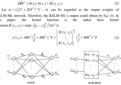
However, in KELM-ML network, there are neither necessity to calculate the hidden layer output nor assign the number of hidden layer nodes, just requiring selecting proper kernel function K u v( , ). The structure of KELM-ML is presented in Figure 1(b). HHT

can be replaced by kernel function, which is HH i jT( , )K x x( ,_{i j}). Kernel matrix definition sees Eq.(2):

( ) ( ) ( , )

  

T

i j i j

HH h x h x K x x (2)

Let  (I C HHT)1Y ,



can be regarded as the output weights of

KELM-ML network. Therefore, the KELM-ML’s output could obtain by Eq. (3). In this paper, the kernel function is the radial basis kernel

functionK x x( , )_{k i} exp( x_kx_i 2 (22)).

1

1 1

( , )

( ) ( ) ( )

( , )

T k

T T T

k

k m K x x

I I

f x HH HH Y HH Y

C C

K x x

 

 

 

  _{ } 

 

 

[image:3.612.107.507.194.475.2]

(3)

Figure 1. Network Structure.

Figure 1. Network Structure.

The output of the KELM-ML network is a q-dimensional real-valued vector, which do not meet the multi-label classification system’s binary output vector requirement. As a result, we need a threshold function t to transfer the KELM-ML network output to binary vector. Refer to references [16], threshold is set as a linear function

* * *

( ) , ( )

t x  a f x b , where a*is a q-dimension vector, b* is the offset. The least

square method can be used to solve this optimization problem as shown in formula (4). For xi, compared the j-th neuron output f xj( )i in output layer with the j-th component

of target value Yi, and if

( )j i

Y is relevant label, add f x_j( )_i into the relevant set Ui of

i

x , or else add f x_j( )_i into the irrelevant set U_i



. ( )s x_i can be considered as a boundary between relevant set and an irrelevant set. So, ( )s x_i can be easily approximated

by(max(U_i) min(U_i)) / 2



* *

* * * 2

{ , } ₁

min ( , ( ) ( ))

m

i i

a b _i

a f x b s x



 



(4) For a test set ' {( , ) |1 x Yi i  i m'} with m' instances, threshold can be

obtained by Eq.(5). Where, Eis a m' 1 dimensional matrix with all element values of

1.

* * ' 1

[[ ( ), _][ , ] ]

 T T

m

t f x E a b (5) As shown in Eq.(5), threshold t is a m' dimensional vector associated with testing set. Then, we pass output f x( )i through threshold t to obtain multi-label classification

results and threshold process method could be seen in Eq. (6):

1 ( ) ( )

( , ) 1, , ' 1, ,

1 ( ) ( )

k i k ii f x t k

finaloutputs k i i m k q

f x t k

 

_  



 (6)

PARALLEL COMPUTING FOR KELM-ML Calculation of KELM-ML Output Weight

In Section 3, the output weight of KELM-ML network is  (I C HHT)1Y .

Consider using Cholesky matrix decomposition method to reduce the computational complexity. The premise of Cholesky matrix decomposition is that the matrix is a symmetric positive definite matrix.

Proof：∵AT (I C HHT T) I C HHT A∴ A is a symmetric matrix.

For an KELM-ML network construct by training set which contains m instances,

the dimension of HHT is m m . Set  be no-zero m-dimensional column vector, then:

  T_A  T(_{I C} _HHT)   T _C T_HHT   2 _C  _HT 2 0

∴ A is a positive definite matrix. In summary, A is a symmetric positive definite matrix.

According to the Cholesky method [2], the matrix A can be decomposed into

T

ALL , in which the L is the lower triangular matrix, and the elements in L are calculated as the Formula (7), where i j, 1, ,m.

1 2 1

1 1

1 ( )

i ii k ik

ij j

jj ij k jk ik

a l i j

l

l a l l i j

     _{ }      





(7)

SinceALLT , A1 ( )LT 1L1. Based on the matrix knowledge, the inverse matrix of the lower triangular matrix is still the lower triangular matrix. LetP L1, P is a lower triangular matrix. p_ij can be obtained by the Eq.(8).

1 0 1 ij ii i i j

p l i j

p  l p i j

So, A1 ( )LT 1L1 P PT (9) Formula (9) shows that the output weight of KELM-ML

 _{(I C HH}T₎1_{Y A Y}1 _{P PY}T

can be calculated only by the matrix product

operation.

Large Matrix Cholesky Decomposition Algorithm

A double type variable takes up 8 bytes on a 64-bit operating system. If size of a matrix is 80000×80000, 80000×80000×8/1024/1024/1024=47.68GB storage space is needed to load whole matrix into memory. Most PCs are unable to load the whole matrix into memory. Therefore, Cholesky matrix decomposition method in Section 4.1 needs to be decomposed and computed in parallel.

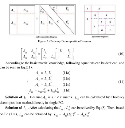
The equation ALLT in Section 4.1, and both two sides of matrix of the equation decomposed into 2×2 block matrices, as shown in Eq.(10) and Figure 2 (a). The original matrix A is a m m square matrix, and A₁₁ is a square matrix of size r r . r is the size of a single PC which can be calculated in the acceptable time (in our experiment set

 200

[image:5.612.95.502.321.735.2]

r ). In Eq. (10), L₁₁ and L₂₂ are still lower triangular matrices.

Figure 2. Cholesky Decomposition Diagram. Figure 2. Cholesky Decomposition Diagram.

 

   

  

   

 

   

     

11 12 11 11 21

21 22 21 22 22

T T

T

A A L L L

A A L L L (10)

According to the basic matrix knowledge, following equations can be deduced, and can be seen in Eq.(11):

 



 

 _



 _{ }



11 11 11

12 11 21

21 21 11

22 21 21 22 22

(11 ) (11 ) (11 ) (11 )

T

T

T

T T

A L L a

A L L b

A L L c

A L L L L d

(11)

Solution of L₁₁. BecauseA₁₁ is a r r matrix, L₁₁ can be calculated by Cholesky decomposition method directly in single PC.

Solution of L₂₁. After calculating theL₁₁, L₁₁1 can be solved by Eq. (8). Then, based

Solution of L₂₂. After changing Eq.(11d) into L L_{22 22}T A₂₂ L L_{21 21}T , L₂₂ can be

calculated by Cholesky decomposition method. If the size of matrix A₂₂ L L_{21 21}T is too large to compute in a single PC, it can be decomposed into small block matrix then recursive solution.

Figure 2 (b) presents the parallel calculation sequence diagram of a 4r-rank square matrix Cholesky decomposition. The number represents the calculation sequence of each sub matrix. The first, third, fifth, seventh matrices are decomposed through using Cholesky method. Calculations of these four block matrices are not parallel. The second blocks, the fourth and the sixth blocks are calculated parallel respectively after calculating completion of the previous block.

EXPERIMENTAL ANALYSES Data Sets and Evaluating Indicator

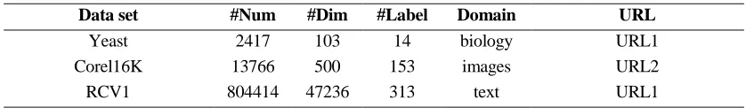
[image:6.612.87.506.468.529.2]

To measure the performance of our approach, three different domain data sets are involved in this paper. The features of data sets are shown in TABLE I. "#Num", "#Dim" and "#Label" are denotes the properties of number of samples, number of features, number of possible class labels respectively. Note that RCV1 (Reuters Corpus Volume 1) uses the "industries:fullsets", which is called "RCV1" for short in this paper. The multi-label learning experimental evaluation indicator adopts the indicators proposed in [12]: "Hamming loss", "One-error", "Coverage", "Ranking loss", these four indicators of lower values, better performance. The experimental results in TABLE III denote with the "↓". The index of "Average precision" the higher the value, the better the performance, the experimental results in TABLE III denote with the "↑”.

TABLE I. FEATURES OF DATA SETS.

Data set #Num #Dim #Label Domain URL

Yeast 2417 103 14 biology URL1

Corel16K 13766 500 153 images URL2

RCV1 804414 47236 313 text URL1

URL1: https://www.csie.ntu.edu.tw/~cjlin/libsvmtools/datasets/ URL2: http://mulan.sourceforge.net/datasets.html

Experimental Results

The experiment compares the performance of KELM-ML algorithm with the existing multi-label classification learning algorithm: Rank-SVM [9], ML-KNN [8], ECC[6]. KELM-ML is deployed on a distributed cluster built on Hadoop-2.7.3

platform. The cluster possesses 4 PC (2.5GHz CPU and 4GB RAM) with Ubuntu 14.10

operating system. Eclipse is adopted as the development tool and Java as the programming language. The initial large matrices are saved as HDFS files. After carrying out the test, for KELM-ML, the optimal kernel parameter 2

2

 _ 

parameter 3

2

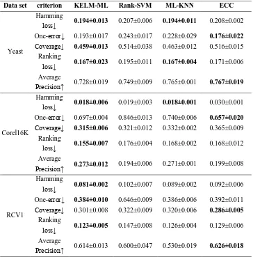
[image:7.612.113.477.231.281.2]

C in Corel16K dataset and RCV1 dataset. Certainly, the parameter selection of KELM-ML algorithm is time-consuming. In terms of ECC, ensemble size is set to be 10, and sample ratio is set to be 67% [6]. The "cross - validation" method is used in the training process. The algorithm average training time are shown in TABLE II, and the time unit is second. Obviously, the training time of KELM-ML algorithm is less than other algorithms. Test set results are presented in TABLE III. According to TABLE III, KELM-ML algorithm in "Hamming loss" and "Ranking loss" indicators gain outstanding performance, and "One-error", "Coverage", "Average Precision" indicators are slightly inferior to the ECC algorithm. In general, KELM-ML algorithm greatly reduces the training time and achieves better overall performance with the supports of parallel computing.

TABLE II. TRAINING TIME OF EACH ALGORITHM (MEAN VALUE).

Data set KELM-ML Rank-SVM ML-KNN ECC

Yeast 0.49 3058 0.32 473

Corel16K 38.16 5974 37.38 947.34

[image:7.612.116.480.313.682.2]

RCV1 126.35 33215 829.20 327.45

TABLE III.RESULTS OF COMPARING ALGORITHM (MEANS±STD).

Data set criterion KELM-ML Rank-SVM ML-KNN ECC

Yeast

Hamming

loss↓ 0.194±0.013 0.207±0.006 0.194±0.011 0.208±0.002 One-error↓ 0.193±0.017 0.243±0.017 0.228±0.029 0.176±0.022

Coverage↓ 0.459±0.013 0.514±0.038 0.463±0.012 0.516±0.015 Ranking

loss↓ 0.167±0.023 0.195±0.011 0.167±0.004 0.171±0.006 Average

Precision↑ 0.728±0.019 0.749±0.009 0.765±0.001 0.767±0.019

Corel16K

Hamming

loss↓ 0.018±0.006 0.019±0.003 0.018±0.001 0.030±0.001 One-error↓ 0.697±0.004 0.846±0.013 0.740±0.006 0.657±0.020

Coverage↓ 0.315±0.006 0.321±0.012 0.332±0.002 0.365±0.009 Ranking

loss↓ 0.155±0.007 0.176±0.004 0.168±0.002 0.168±0.012 Average

Precision↑ 0.273±0.012 0.194±0.006 0.271±0.001 0.199±0.008

RCV1

Hamming

loss↓ 0.081±0.002 0.102±0.007 0.089±0.002 0.092±0.006 One-error↓ 0.384±0.010 0.646±0.009 0.386±0.006 0.392±0.011 Coverage↓ 0.301±0.008 0.322±0.009 0.320±0.006 0.286±0.005

Ranking

loss↓ 0.123±0.005 0.147±0.008 0.126±0.004 0.129±0.006 Average

CONCLUSIONS

In this paper, a multi-label learning algorithm KELM-ML is designed based on the kernel extreme learning machine, and an adaptive threshold function is set up. Specially, the KELM-ML output weight is obtained with the application of the Cholesky Matrix Decomposition method. The inverse problem of large matrix is solved by matrix block method. Finally, the comparison experiment shows that KELM-ML has better effect and fast training time.

ACKNOWLEDGEMENT

This work was supported by the National Science Foundation of China under Grant No.61672159 and 61571129, the Fujian Collaborative Innovation Center for BigData Application in Governments, the Technology Innovation Platform Project of Fujian Province(Grant No.2009J1007 and 2014H2005).

REFERENCES

1. Sun X., Wang J., Jiang C., Xu J., Feng J, Chen S. S., and He F. 2015. “ELM-ML: Study on Multi-label Classification Using Extreme Learning Machine,” presented at the proceedings ELM-2015, 2:107-116, December 5-17, 2015.

2. Huang G. B., Zhou H., Ding X., and Zhang R. 2012. “Extreme learning machine for regression and multiclass classification,” IEEE Transactions on Systems Man and Cybernetics Part B Cybernetics A Publication of the IEEE Systems Man & Cybernetics Society, 42(2):513-29.

3. Zhang X. D. 2005. Matrix analysis and application. Beijing: Tsinghua University Press, pp.225-227. 4. Scardapane S., Comminiello D., Scarpiniti M., and Uncini A. 2015. “Online Sequential Extreme Learning Machine With Kernels,” IEEE Transactions on Neural Networks and Learning Systems, 26(9):2214-2220.

5. Zhang X., Wang H. L. 2011. “Incremental regularized extreme learning machine based on Cholesky factorization and its application to time series prediction,” Acta Physica Sinica, 60(11):2509-2515. 6. Zhou X. R., Wang C. S. 2016. “Cholesky factorization based online regularized and kernelized

extreme learning machines with forgetting mechanism,” Neurocomputing, 174(1):1147-1155. 7. Boutell M. R., Luo J., Shen X., and Brown C.M. 2004. “Learning multi-label scene classification,”

Pattern Recognition, 37(9):1757-1771.

8. Hüllermeier E., Fürnkranz J., Cheng W., and Brinker K. 2008. “Label ranking by learning pairwise preferences,” Artificial Intelligence, 2008, 72(16-17):1897-1916.

9. Read J., Martino L., and Luengo D. 2014. “Efficient Monte Carlo Methods for Multi-Dimensional Learning with Classifier Chains,” Pattern Recognition, 47(3):1535-1546.

10. Al-Salemi B., Noah S. A. M, and Aziz M. J. A. 2016. “RFBoost: An Improved Multi-Label Boosting Algorithm and Its Application to Text Categorisation,” Knowledge-Based Systems, 103:104-117. 11. Zhang M. L., Zhou Z. H. 2007. “Ml-kNN: A lazy learning approach to multi-label learning,” Pattern

Recognition, 40:2038-2048.

12. Elisseeff A. E., Weston J. 2002. “A Kernel Method for Multi-Labelled Classification,” Advances in Neural Information Processing Systems, 14:681-687.

13. Mahmood S. F., Marhaban M. H., Rokhani F. Z., Samsudin K., and Arigbabu O.A. 2016. “FASTA-ELM: a fast adaptive shrinkage/thresholding algorithm for extreme learning machine and its application to gender recognition,” Neurocomputing, 2016219(C):312-322.

15. Iosifidis A., Tefas A., and Pitas I. 2015. “On the kernel Extreme Learning Machine classifier,”

Pattern Recognition Letters, 54(P1):11-17.