Planning VANET infrastructures to

Planning VANET infrastructures to

improve

safety awareness in curved roads

Hossein GHAFFARIAN, Mohsen SORYANI, Mahmood FATHY‡

(School of Computer Engineering, Iran University of Science and Technology, Narmak, Tehran, P.O. Box 13114-16846, Iran) E-mail: [email protected]; [email protected]; [email protected]

Received Mar. 26, 2012; Revision accepted Aug. 20, 2012; Crosschecked

Abstract: We analyse the effect of using VANET on accident avoidance. As shown in our analysis, a higher frequency of safety

packets can prevent accidents, even for high speed vehicles and dense roads. In addition, to overcome connectivity problems in blind crossing situations, a genetic algorithm (GA) based method for VANET infrastructure planning is also presented. The proposed approach tries to remove coverage sight holes in low sight distance cases in a traveling path in the road. In such places, drivers might not have enough sight for proper action and also environmental obstacles prevent direct communication between vehicles. Furthermore, curved roads affect mobility. Simulation results show that the density of vehicles is increased right before a curve and is decreased after that. Therefore, in this kind of road, a high frequency of packet generation may not act well in accident avoidance. The method proposed in this paper tries to cover such places considering the lowest safety distances according to traffic theory. For this, the road must be covered directly by infrastructure. Therefore, the problem is to find the best number and also positions of road side units. Using GA, the algorithm minimizes the summation of total uncovered and overlapped points in the roads which are covered by more than one antenna. Simulation results on a real road map confirmed the capabilities of the pro-posed approach.

Key words: VANET, Infrastructure, Traffic theory, Minimum safety requirement, Genetic algorithm doi:10.1631/jzus.C1200082 Document code: A CLC number:

1 Introduction

The Institute of Transportation Engineers define traffic engineering as the application of technology and scientific principles for the planning, functional design, operation, and management of facilities for any mode of transportation in order to provide for the safe, rapid, comfortable, convenient, economic, and environmentally compatible movement of people and goods (Pline, 1999). As mentioned in this definition and other similar definitions, the primary objective of traffic engineering is safety. Studies by the U.S. De-partment of Transportation show that the three largest crash types (rear-end, intersection, and road

depar-ture) account for nearly 75% of all crashes (U.S. Department of Transportation, 1999). These studies show that driver inattention plays a key role in dents. Based on an AHSRA report, 65.1% of acci-dents happen just because of inattention to the for-ward view (AHSRA Japan, 2001). Adler (2006) re-ported that different studies show that in 69% of cases, crashes happen because of the absence of critical and necessary information for drivers in ap-propriate time. Formal active safety systems like camera vision and radars cannot provide information about situations beyond other vehicles. Vehicular ad-hoc network (VANET), as a radio communication system, solves this problem. Vehicles which are not in the sight distance of each other could communicate using communication capabilities of intermediate vehicles.

Journal of Zhejiang University-SCIENCE C (Computers & Electronics) ISSN 1869-1951 (Print); ISSN 1869-196X (Online)

www.zju.edu.cn/jzus; www.springerlink.com E-mail: [email protected]

‡ _{Corresponding author}

* _{This work is supported by Iranian Research Institute for ICT} © Zhejiang University and Springer-Verlag Berlin Heidelberg 2012

The fundamental goal of VANET is improving safety in roads. For this, VANET nodes (vehicles) can communicate with each other without any need for extra infrastructure like road side units (RSU) or any type of base stations. For example, Kato et al. (2002) present a vehicle control algorithm which works ac-cording to the cooperation between following vehi-cles based on VANET. Their proposed approach enables groups of vehicles to be merged together or separated from each other. Taleb et al. (2010) propose a collaborative collision avoidance system based on VANET. Yousefi et al. (2008a) enumerate effective range and beaconing rate as key metrics for per-formance evaluation of safety applications in VANET.

The main drawback of VANET is the deploy-ment cost. It is necessary to have an acceptable number of well equipped vehicles with VANET tools. Equipping VANET with infrastructure, as a new as-pect, vehicles communicate across an RSU with out-side nodes on the Internet. Therefore, value-added services, e.g., entertainment, online games, adver-tisements and file sharing, become available by using VANET. New services can add more attraction for data service providers toward VANET. The main issue in this case is the vehicle localization across the road to deliver data from the best RSU. Saleet et al. (2010) propose a region based location service man-agement protocol for VANETs which has a limited query and response overhead on the network. In (Cruces et al., 2009), some planning roadside infra-structure strategies are proposed for information dis-semination. The proposed approaches try to maxi-mize the overall service time usage by planning for k RSUs in a region or city. Their conclusion shows that planning for RSUs in intersections provides the best answer. On average, vehicles spend more time in intersections than other parts of roads. Although these new services can make VANET infrastructure plan-ning more economical, they should not bend attention from safety into other areas. Therefore, RSUs can be used to improve safety as well.

In this paper, first we analyse the efficiency of VANET to avoid accidents. For this, we focus on IEEE 802.11p standard and rate of generating safety packets. In VANET equipped vehicles, an engine control unit can request the activation of the break as soon as it detects dangerous situations based on

re-ceived data. We extend our analysis to a wide range of speeds, vehicle density in the road and different packet generation rates. Furthermore, we propose a new GA-based approach to cover blind crossing ar-eas, e.g., curved roads and even intersections. Simu-lation results show that in curved roads, traffic density is affected by the curve. In sparse traffic densities, the connectivity probability of nodes is decreased. Therefore, in blind crossing cases like curved roads and intersections, non-line-of-sight communication using infrastructure is necessary for safety. Our pro-posed approach focuses on indirect message propa-gation using infrastructure. We have implemented our approach in MATLAB and used it to cover a real curved road.

The remainder of this paper is organized as fol-lows: in Section 2, a literature review on minimum safety distance requirements is prepared. Our analysis about the efficiency of VANET in accident preven-tion is presented in Secpreven-tion 3. The main focus of this paper is keeping connectivity between following vehicles to avoid collisions in the curved roads. In Section 4, through simulations, we show the effect of curved roads on the vehicle density. A GA-based approach for covering curved roads to meet safety requirements is introduced in Section 5. In Section 6, results of the proposed method in a real curved road are presented. Finally, the paper is concluded in Sec-tion 7.

2 Literature review on minimum safety dis-tance requirements in traffic theory

Before talking about the effect of VANET on safety, it is necessary to have a primary understanding about the safety conditions in roads. Therefore, in this part, we review the main formulas and challenges in safety in traffic engineering (Roess et al., 2004). 2.1 Road users

There are several characteristics that affect road users. Among them, field of vision and percep-tion-reaction time (PRT) are the most important ones. Field of vision is related to the area in which drivers can see and detect objects. The Institute of Trans-portation Engineering in USA has defined three dis-tinct fields for stationary persons (Dewar, 1999).

However, as speed increases, these fields become narrow. Therefore, risk of accidents increases. PRT is the time in which a driver detects an unexpected ob-ject or condition in his or her field of vision, tries to identify it, makes a decision and finally reacts to it. Based on studies of the American Association of State Highway and Transportation Officials (AASHTO), in 90% of cases, drivers react in less than 2.5 s (Offi-cials, 2001). Nevertheless, there are other measured domains for PRT too, e.g. 0.75-1.5 second is used in (Yang et al., 2004) which is repeated in (Taleb et al., 2010). Using kinematic theory, reaction distance, the distance in which a vehicle travels during PRT, can be calculated by dPRT=vt, where dPRT is the reaction dis-tance (m), v is the initial speed of the vehicle (m/s) and t is the reaction time (s). According to the AASHTO recommendation, this formula is summa-rized as dPRT=2.5v . Pedestrian behavior, drug im-pacts and vehicle characteristics have important ef-fects on driving, which need social investigations and more complicated research. Therefore, we ignore them in this paper.

2.2 Acceleration and deceleration

Acceleration and deceleration have great im-pacts on safety. Acceleration is related to the vehicle type and weight-to-horsepower ratio. However, de-celeration is related to the braking system character-istics. Acceleration/deceleration distance can be computed as follows: 2 2 / ₂ i f a d v v d a   (1)

where da/d is the acceleration/deceleration distance (m), vi is the initial speed (m/s), vf is the final speed (m/s) and a is the acceleration rate (m/s2). In breaking cases, to express equation (1) in terms of the coeffi-cient of forward rolling or skidding friction, F, where

F=a/g, and g is the acceleration due to gravity, 9.8

m/s2, the deceleration distance can be addressed as follows: 2 2 30( 0.01 ) i f d v v d F G    (2)

where dd is the deceleration distance (m), F is the

coefficient of forward rolling or skidding friction and

G is the grade (%). The standard deceleration rate,

which covers 90% of cases, is 3.4 m/s2 (Roess et al., 2004). Therefore, equation (2) can be summarized as follows: 2 2 30(0.347 0.01 ) i f d v v d G    (3)

The total stopping distance, which is critical in safety applications, can be calculated as follows:

2 2 2.5 30(0.347 0.01 ) total PRT d i f i d d d v v v G       (4)

Equation (4) is the base of safe stopping sight distance, decision sight distance calculations and other related distance intervals, especially in inter-sections and traffic lights. Another criterion is the safe stopping sight distance between two moving vehicles. While the vehicle in front (Ci) decelerates, the min-imum required distance for safe stopping of the ve-hicle in behind (Ci-1) can be calculated as follows:

1 1 i total PRT i i d d d d      ₍₅₎ where 1 i PRT

d

2.3 Low sight distance in horizontal curves

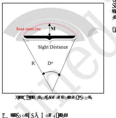
Horizontal curves are common in different roads, especially in highways, sub-urban and rural roads. The severity of these curves is related to the designed degree of curvature. As mentioned, the minimum sight distance has a great effect on safety. Therefore, road designers must be aware of this im-portant issue in road design. Because of roadside objects, the sight distance is limited on horizontal curves. According to Fig. 1, the middle oriented of the horizontal curve must be enough to provide the least required sight distances as follows (Roess et al., 2004): 1 cos 200 total d D M R_  _ __     (6)

unedited

where M is the minimum required middle oriented (m), R is radius of the curvature (m), dtotal is the total stopping distance and D is degree of the curvature.

In some places like mountains and valleys, reaching the minimum M and sight of distance is difficult and costly. In such places, roads are designed in a spiral while low sight of distance and safety recommendations may be ignored. Another special case of dangerous positions is intersections. While drivers move straight, the minimum sight distances for crossing vehicles are not met because of buildings, trees and other environmental obstacles. Such points are great potential points for accidents. Although designers try to inform drivers about intersections and possible dangers using traffic signs and marks, these are not enough. It seems that VANET infrastructure can provide more information about road crossings that drivers approach blindly. In the next section, we analysed the effects of VANET for improving safety.

Fig. 1 Sight restriction on horizontal curves

3 Effect of VANET on safety

In this section, we analyse the effect of VANET in accident avoidance. In (Busson et al., 2011) the authors analyse the possibility of an accident for consecutive vehicles. Although they focus on mul-ti-hop message propagation to avoid an accident, safety information has local value. Therefore, in this paper, we analyse the effect of VANET on safety, using single hop message propagation.

To answer safety issues in the roads, IEEE has proposed IEEE 1609 series of standards (IEEE Std. 1609.1-2007, IEEE Std. 1609.2-2007, IEEE Std. 1609.3-2007, IEEE Std. 1609.4-2007) for Wireless Access in Vehicular Environments (WAVE) com-promised with IEEE 802.11p (IEEE Std. P802.11p/ D3.0, 2007). The IEEE 802.11p standard is based on IEEE 802.11e (Alcaraz et al., 2009). The MAC layer of IEEE 802.11p has two modes: contention-based mode and contention-free mode. The former is related to the situation in which sender nodes contend with each other to get a chance for transmission. In the latter, a polling mechanism is used. Because of the delay overhead of polling and the need for an external coordinator, the second method is unsuitable for use in emergency data propagation. In IEEE 802.11p, the channel is divided into 100 ms time intervals. Each time interval is divided into two 50 ms sub-intervals: Central Control Channel (CCH) and Six Service Channels (SCH) (Mišić et al., 2011). Safety messages can only be transmitted in CCH intervals with default frequency of 10 Hz. However, during congestion in the channel, this rate is decreased.

Before continuing the analysis, we make some assumptions as follows:

- Suppose that a group of tandem vehicles with the same specifications and VANET equipment move on a road.

- Suppose that all of the tandem vehicles have localization capability, e.g. GPS, to detect their current positions.

- Suppose that the network channel is perfect. There is no packet corruption or packet loss in the network. However, adding effect of channel fading and loss models, like Nakagami (Naka-gami, 1960), in experiments is straight forward. - dtotal in equation (5) is discretized in sections

with 1 cm length.

- Also, suppose that distribution of vehicles in the road is Poisson with inter vehicle distance of λ meters (λ=1000/density).

- According to (Yousefi et al., 2008b), lane width with respect to the communication range of ve-hicles is negligible. Therefore, we can simply replace a multi-lane road with a single-lane road.

According to Section 2, an accident could hap-pen if the distance between two tandem vehicles is

less than dtotal in equation (5). In such a situation, the driver has little chance to have sufficient reaction time to avoid upcoming accidents. For a given λ and dtotal, the Cumulative Distribution Function (CDF) of the Poisson distribution (equation 7) returns the possibil-ity that the distance between two tandem vehicles, with specified speeds, in the road, with a specific density, is less than or equal to dtotal. Therefore, this possibility can be interpreted as the possibility of occurrence of an accident in the road.

0 ( , ) ( ) ! total d i total total i F d P d e i         



Using this method, we can divide a chain of n vehicles into n-1 different two tandem vehicles to find the possibility of an accident between them.

To reduce the possibility of an accident, we need to restrict dtotal in equation 5. Although di and di-1 are related to the velocity of the vehicles, dPRT is reduci-ble. In VANET enabled vehicles, automatic breaking in case of detecting a hazard can reduce PRT. Higher

packet rates mean lower interval time between two consecutive packets and therefore, shorter PRT.

Fig. 2 shows the possibility of an accident for different packet rates. This figure is drawn based on equations (5) and (7). In this figure, the speed dif-ference between two tandem vehicles ranges from 15 m/s to 40 m/s. Also, the density of vehicles in the road is between 8 vehicles per kilometer to 13 vehicles per kilometer. These density rates can satisfy minimum safe distance between two tandem vehicles with maximum deceleration rate of -10 m/s2. As we can see, lower data rates, higher speeds and higher densi-ties have direct relation with increasing possibility of an accident. Comparing results of figures 2.a/b with 2.e/f shows the direct effect of the number of gener-ated packets, especially in congested situations. If we assume that PRT for humans is one second, then the possibility of an accident for a vehicle under human control is equal to the case of sending one packet per second in VANET.

4 Investigating the effect of curved roads on density of vehicles

To study the effect of the curved road on the density of vehicles, we have set up a simulation using MATLAB software. The simulated area consists of a curved road with two same direction lanes and 2 km length. Speed limitations in the road, vmin, vavg and

vmax, are equal to 60 km/h, 75 km/h and 90 km/h, respectively. If the distance between two following vehicles became less than half of the safety distance, the follower must reduce its speed. Otherwise, each vehicle could accelerate or decelerate in the range of [-10, +10] m/s2 freely (the probability of acceleration is 0.15, the probability of deceleration 0.15 and in 70% of situations vehicles do not change their ve-locities). Also, PRT is 2.5 s.

Suppose that there is a curve placed in the mid-dle of the road with its center placed in the 1000th meter of the road, with minimum sight distance of 50 meters. Vehicles must reduce their speed to vmin 100 meters before the center of the curve. They are free to accelerate 50 meters after the center of the curve. In addition, takeover is forbidden along the road. The road grade G is 4. Simulation time is 4000 seconds in which we omitted the results of the first and last 200 s.

In other words, we have analysed the results of 3600 s or 1 hour of simulation. The simulation results have been updated and analysed every 0.1 s during the simulation. The simulation is run 100 times.

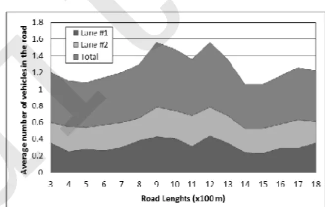
Fig. 3 shows the average density along the road. To remove the side effects of the two ends of the road, the results of the first and the last 200 m of the road is not present in this figure. As shown in the figure, although the average density along the road is somewhat fixed, in the distance between 800-1300 m, we have two big fluctuations. The first one occurred because of the effect of the curve in the road on the mobility of vehicles. The vehicles have to reduce their speed before the curve, pass the curve and after that they are free to increase their speed. The second fluctuation occurred because of the effect of vehicles in front of them. These speed changes cause backlogs before and after the curve.

Fig. 3 Vehicle density analysis along the curved road

Fewer numbers of vehicles in the area near to the curve mean less connectivity. In addition in the curved roads, obstacles can prevent direct commu-nication between tandem vehicles. Therefore, in the case of low density, even higher data rates cannot solve the safety problem. To cover this problem, in curved roads, infrastructure can relay safety messages between vehicles. In the next section, we propose a GA based method to find a suitable position for an-tenna in curved roads.

5 The proposed GA-based planning algo-rithm

In this section, we introduce a GA-based plan-ning strategy for minimum cost deployment of

VANET infrastructure. Genetic algorithm is one of the well-known optimization tools. The proposed method is introduced to prepare the best coverage in the road positions which do not provide enough sight distances as safety applications require. Proposed approaches like (Sepulcre et al., 2011), focus on re-liability of 99.99% in accident avoidance. This reli-ability is achieved if and only if the follower vehicle receives at least one safety packet in proper time be-fore the break. Therebe-fore, planning strategies like (Abdrabo et al., 2011), cannot react well in such cases. The method in (Abdrabou et al., 2011) is based on satisfying maximum tolerable delay bounds of applications, not safety considerations.

If there is not minimum density in the road, as (Mohimani et al., 2009) analyses, the connectivity between vehicles is broken. Therefore, in the plan-ning strategy, we follow the direct communications strategy between vehicles and antennas in the curved roads. We propose full coverage of such areas, using VANET infrastructure. Deploying infrastructure is costly; therefore, finding the least number of required antennas is important.

The proposed method has three steps as shown in Fig. 4. The first step is preprocessing. In this step, the map of a road is injected into the software or proc-essed manually. This map only contains the area with minimum safety distance requirements. Based on the height of antennas, the map is divided and colored into three regions: road, roadsides with height lower than the antenna and roadsides with height higher than the antennas. In the second step, the processed map is analysed according to the communication range of the antennas and environmental obstacles in the direct path of signal propagation. The output of this step is the number of antenna with minimum cost to cover safety requirements in the road. In the last step, the best positions for the selected number of antennas are chosen.

Fig. 4 Steps of the proposed GA-based planning algorithm

5.1 Preprocessing

In the first step, a map of the area is processed based on the chosen height of the antenna. The height of an antenna has important effects on signal

propa-gation. Although short antennas have problems in data dissemination with respect to environmental obstacles, tall antennas need more transmission power. Furthermore, in some situations, e.g. inter-sections or mountainous roads, obstacles are long and elevated. For the given height of an antenna, the map is colored in black, for regions in which signals can-not propagate in them, gray, for roadsides which do not disturb dissemination, and white, for the road area which must be covered by direct signals of antennas. 5.2 Choosing the right number of antennas

Let us assume that we deal with an optimization problem to minimize a cost function as follows:

1

( ) ( ,..., )n

f x  f x x ₍₈₎

subject to some conditions. In the first step, we need to define x1, x2, …, xn. As mentioned before, because of a low degree of connectivity, we are looking to cover the curved area such that vehicles could com-municate with RSUs directly. Therefore, we need at least two inputs: a map of the road and a detailed coverage area of each antenna. For simplicity and also minimizing the cost of antenna, in this paper, we only focus on omnidirectional antennas. Using this type of antennas, we only need to know the communication range of the antenna and its position to calculate the coverage.

For the cost function, we need to determine the elements that affect the cost. Based on our strategy for direct communication between RSUs and vehicles, uncovered points by antennas are against our strategy. Furthermore, reducing the installation cost is impor-tant too. For this reduction, we need to avoid over-lapped covered points as much as possible. Based on these factors, we define our cost function C for minimization as follows:

min( )

C    





where α and β (α, β>0) are weights of summation of uncovered points ϑ and summation of overlapped covered points ѱ, respectively.

To choose the best number of antennas, GA is used. The area of a curved road is not convex. It consists of multiple consecutive curves in small areas. Therefore, using mathematical optimization ap-proaches like convex optimization or linear

gramming is impossible or difficult in such condi-tions. In addition, the proposed ILP approaches for sensor placement, like (Chakrabarty et al., 2002; Sahni et al., 2005; Xu et al., 2007; Osais et al., 2009), have a time complexity problem. They fail to return the final answer in an acceptable length of time. For example, in a 2020 grid field, the proposed model of (Sahni et al., 2005) returns the answer after 14 hours (Osais et al., 2009). GA is a powerful, robust and flexible optimization tool. It can be easily modi-fied for different problems, while it can tolerate noisy functions as well (Sivanandam et al., 2008). The main inputs of GA are genomes and a fitness function. As shown in Fig. 5, the structure of genomes contains position information of antennas. In this structure, (Xk,Yk) is the position of antenna k. Here, we suppose that all antennas are similar. Therefore, for memory saving, we use communication range as a global variable, not a local variable in the structure of the genome.

Fig. 5 Common structure of the used genomes

The second important input is the fitness func-tion. This function provides the fitness value for each offspring. We use the proposed cost function C in equation 9 as our selected fitness function. The best answer is the case with minimum fitness value.

Based on the position information in the ge-nome, antennas are placed on the processed map. Then, according to the colored map, the covered area of each antenna is determined. If a point in the road, presented by white color, remained uncovered, it implies a negative point. In addition, if two antennas become closer than twice the communication range, some inappropriate overlapped points appeared. Therefore, the summation of uncovered points and overlapped covered points is calculated as a negative score for the genome.

To calculate these negative points, in each round two matrices with the same size of the original image is prepared. In the first matrix, the cells corresponding to road points in the map take value 1 and other cells take value 0. To complete this matrix, we prepare a black and white image using the threshold equal to 0.6. Therefore, any point which is not placed on the

road takes value 0. If a cell is covered by an antenna and its value is not 0, its value is changed into 0.5. Cells in the second matrix have value 0 at first. If a point is covered by an antenna, its corresponding cell value is incremented to show the possible overlaps. To check the environment effects on data dissemina-tion of each antenna, we create another black and white copy of the map using the threshold equal to 0.2. Therefore, gray points are changed into white. The data is disseminated if and only if there are not any black points in its path.

By running different iterations of GA, new off-spring are generated by crossover and recombination of old genomes. Moreover, some offspring can be mutated and make new generations. Genomes with better fitness values have more chances to remain in the current generation for the next round of the algo-rithm. The selection algorithms do not select the best options only because such a selection strategy can cause the algorithm to produce sub-optimal answers.

The GA-based algorithm must be run with the different number of antennas and communication ranges. Then, the best choice for the required number of antennas can be determined. It is recommended to choose the right number with respect to the backbone facilities. Although selecting the case with lower fitness value, lower number of antennas and higher communication ranges can be the best choice, this option causes difficulties for backbone connectivity between antennas.

5.3 Finding best positions for antennas

The final step of the planning algorithm is to find the best places for antennas. For this, there are two approaches. First, in the second step, position infor-mation is gathered and after choosing the number of antennas, their positions are extracted too. Second, after selecting the best values for the number of an-tennas and communication range, the GA-based al-gorithm is run again to choose the best positions for deployment. Selecting the first approach can reduce the time for decision making.

Table 1 GA running parameters

Parameter Value

α 1, 1, 3

β 1, 3, 1

Maximum number of simulations 5

Maximum population size 50

Maximum generation size 50

Maximum Iterations 1000

Maximum number of iterations without any change in the best

fitness value 5

Cross over probability 0.7

Mutation probability 0.03, equation (10)

Selection function Roulette wheel

Crossover function 0.2 Gen1+0.8Gen2

(a)

(b)

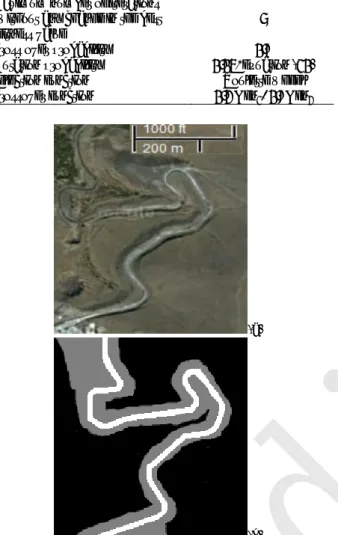
Fig. 6 The selected curved road for coverage; the entrance road of Tuyserkan, Hamedan, Iran (a), satellite map (b), the map after Preprocessing

5.4 Drawbacks of GA

Although genetic algorithm can solve compli-cated optimization problems, it suffers from some unwanted problems. The main negative point of GA is its running cost. GA consumes much memory and time to prepare responses. Although selecting more clear and restricted options can improve this, it can decrease the chance of finding better answers. An-other drawback of GA is that there is not a well- de-fined way to choose the best algorithms for mutation, crossover and selection functions (Sivanandam et al., 2008). As presented in (Eiben et al. 2003), there is not a specific and exact approach for parameter control in GA. Testing different setups to establish a good al-gorithm design, implies a semi-exponential number of runs.

6 Performance evaluation of the proposed method

In this part, first we present simulation pa-rameters and then we investigate the performance of the proposed approach via different simulations. 6.1 Simulation setup parameters

To test the abilities of the proposed GA-based covering algorithm, an image from the entrance road of Tuyserkan (Hamedan, Iran) is selected, which is shown in Fig. 6a. This figure is extracted from Google’s maps website. This image has been pre-processed manually using geographical information and 2-meter height antennas (Fig. 6b). We have im-plemented the rest of the process in MATLAB. The selected GA parameters are shown in Table 1. We repeat simulations five times for each case with a maximum of 1000 iterations for each case. Five rep-etitions are used to avoid unwanted local minima in the final results. The best results in these repeated simulations are selected as the final answer of the algorithm.

Simulations are repeated in three different series. The selected values of α for these series are 1, 1 and 3 and the selected values for β are 1, 3 and 1. A larger α to β ratio means that the uncovered points have a greater impact than the overlapped covered points in the deployment, while bigger β to α ratio means that the impact of the overlapped covered points is greater than the impact of the uncovered points. The selected values in this paper are arbitrary, while readers can choose other values based on their interest. Maximum generation size and maximum population size are limited to 50 cases. Although increasing these sizes can improve the probability of having better results, this makes extra processing time and memory over-head. We have used a single point crossover function with probability of 0.7. Adding further crossover points reduces the performance of the GA (Sivanan-dam et al., 2008). The selected crossover function is 0.2Gen1+0.8Gen2. Furthermore, the selection func-tion is a roulette wheel which is one of the tradifunc-tional and commonly used GA selection techniques (Si-vanandam et al., 2008).

One of the methods used for parameter controls in GA is changing the mutation step size (Eiben et al. 2003). In this paper, we have used two approaches for

this. In the first approach the mutation probability is fixed to 0.03. In the next approach, based on (Eiben et

al. 2003), we have used the following equation to

calculate the mutation probability dynamically, dur-ing the run time.

(0, ( )) p p M initM    t ₍₁₀₎ where ( ) 1 0.9t t T    (11)

In these equations, Mp is the mutation probabil-ity, initMp is the initial mutation probability (equal to 0.03 in this paper), N() is the normal distribution function with mean equal to zero and standard devia-tion equal to σ, t is the current generadevia-tion iteradevia-tion number varying from 1 to T, and T is the maximum generation iteration number (1000 in this paper).

In the rest of the paper, we call the former proach (fixed mutation probability) the primary ap-proach and the latter as the adaptive apap-proach. 6.2 Coverage of the curved road

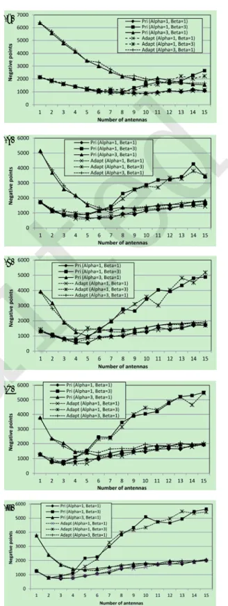
For performance evaluation, we have changed the antennas’ propagation radius from 100 meters to 500 meters with steps of 100 meters. Fig. 7 depicts the results of calculating the antenna locations with minimum negative points. As shown in this figure, the trend of the presented results in the graph is not smooth and uniform. This happens since GA only prepares sub-optimal results. Furthermore, the two defined approaches follow a similar trend. However, most of the time, the trend of the adaptive approach is smoother than the trend of the primary approach. This happens because there are more possibilities of mu-tation in the first rounds of the second approach.

Figs. 7 c/d/e show the effect of increasing the transmission range. As shown in this figure, the dif-ference of the results between different cases with 300 m, 400 m and 500 m transmission range antennas is little. Selecting antennas with a larger transmission range depends on the curved road. If the road has lots of curves with short minimum sight distances, se-lecting smaller transmission range is better; other-wise, a larger transmission radius is considered.

Readers can tune the cost function using α and β, based on their requirements. If they are looking for a full coverage, they can increase the value of α. If they

Fig. 7 Results of selecting best places using antennas with 100 m (a), 200 m (b), 300 m (c), 400 m (d), and 500 m (e) propagation radius (a) (b) (c) (d) (e)

unedited

are looking for using the minimum possible antennas, they can focus on β. The proposed cost function in equation 9 is a general function. Furthermore, the reader can select the transmission range based on the map of the road to examine the effects of curves and obstacles on the effective transmission range of an-tennas.

To show the efficiency of the proposed method, in Fig. 8, we show the selected positions for de-ployment using the primary approach with 100/200 m communication range of antennas. As mentioned before, our criterion for selecting the best number of antennas in this paper is equation 9. Based on Fig. 7, the results of the deployment in adaptive approach are similar to the primary approach; therefore, we do not show their selected points here.

7 Conclusions

Safety is an important goal in ITS and VANET. In this paper, we have shown the effect of VANET in accident avoidance. As results show, using VANET with high rates of safety packets effectively reduces the possibility of accidents, even in high speeds and low inter distance between tandem vehicles. In addi-tion, a novel GA based method was proposed to cover curved roads using VANET infrastructure. In curved roads, there is not enough sight distance for drivers. Furthermore, environmental obstacles prevent direct communication between vehicles. Therefore, the possibility of an accident in such points increases. To solve this problem, we have proposed to plan and install VANET infrastructure in curved roads. The proposed algorithm tries to minimize the summation of uncovered areas and multi-covered areas. Simula-tion results show the abilities of the algorithm. Working on 3D map processing is scheduled as future work.

References

Abdrabou, A., Zhuang, W., 2011. Probabilistic delay control and road side unit placement for vehicular ad hoc net-works with disrupted connectivity. IEEE J. Selected

Ar-eas in Com., 29(1):129-139.

Adler, C. J. 2006. Information dissemination in vehicular ad hoc networks. MS Thesis, University of Munich. Advanced Cruise-Assist Highway System Research

Associa-tion (AHSRA) Japan, 2001. Outline of the Primary Re-quirements of Advanced Cruise-Assist Highway Sys-tems.

Alcaraz, J. J., Alonso, J.V., Haro, J. G., 2009. Control-based Scheduling with QoS Support for Vehicle to Infrastruc-ture Communication. IEEE Wireless com., 16(6):32-39. Busson, A., Lambert, A., Gruyer, D., Gingras, D., 2011.

Analysis of Intervehicle Communication to Reduce Road Crashes. IEEE Trans. on Veh. Tech., 60(9):4487-4496. Chakrabarty, K., Iyengar, S. S., Qi, H., Cho, E., 2002. Grid

Coverage for Surveillance and Target Location in Dis-tributed Sensor Networks, IEEE Trans. on Comp.,

51(12):1448-1453.

Cruces, O. T., Fiore, M., Casetti, C., Chiasserini, C. F., Ordi-nas, J. M. B., 2009. A Max Coverage Formulation for Information Dissemination in Vehicular Networks. IEEE WIMOB. Marrakech, Morocco, p.154-160.

Dewar, R., 1999. Road users: Traffic Engineering handbook. 5th _{edition. Washington DC: Institute of transportation}

engineering.

Eiben, A. E., Smith, J. E., 2003. Introduction to Evolutionary Computing, Berlin, Springer.

Fig. 8 Selected points for installing the antennas with 100 m transmission range covering with 10 antennas in the case α=1 & β=1 (a), 8 antennas in the case α=1 & β=3 (b), and 15 antennas in the case α=3 & β=1 (c), and the an-tennas with 200 m transmission range covering with 5 antennas in the case α=1 & β=1 (d), 4 antennas in the case α=1 & β=3 (e), and 6 antennas in the case α=3 & β=1 (f)

(a) (b)

(c) (d)

IEEE Std. 1609.1-2007, 2007. IEEE Trial-Use Standard for Wireless Access in Vehicular Environments (WAVE)— Resource Manager.

IEEE Std. 1609.2-2007, 2007. IEEE Trial-Use Standard for Wireless Access in Vehicular Environments (WAVE)— Security Services for Applications and Management Messages.

IEEE Std. 1609.3-2007, 2007. IEEE Trial-Use Standard for Wireless Access in Vehicular Environments (WAVE)— Networking Services.

IEEE Std. 1609.4-2007, 2007. IEEE Trial-Use Standard for Wireless Access in Vehicular Environments (WAVE)— Multi-Channel Operation.

IEEE Std. P802.11p/D3.0, 2007. Draft Amendment for Wire-less Access in Vehicular Environments (WAVE). Kato, S., Tsugawa, S., Tokuda, K., Matsui, T., Fujii, H., 2002.

Vehicle Control Algorithms for Cooperative Driving with Automated Vehicles and Intervehicle Communications.

IEEE Trans. on Int. Trans. Sys., 3(3):155-161.

Mišić, J., Badawy, G., Mišić, V.B., 2011. Performance Char-acterization for IEEE 802.11p Network with Single Channel Devices. IEEE Trans on Veh Tech., 60(4):1775- 1787.

Mohimani, G. H., Ashtiani, F., Javanmard, A., Hamdi, M., 2009. Mobility Modeling, Spatial Traffic Distribution, and Probability of Connectivity for Sparse and Dense Vehicular Ad Hoc Networks. IEEE Trans on Veh Tech.,

58(4):1998-2007.

Nakagami, M., 1960. The M-Distribution, a General Formula of Intensity of Rapid Fading, Symposium of Statistical Methods in Radio Wave Propagation, p. 3-36, University of California, Permagon Press.

Officials, American Association of State Highway and Transportation. 2011. A policy on geometric design of highwasy and streets. 4th _{edition, Washington DC.}

Osais, Y., St-Hilaire, M., Yu, F. R., 2008. Directional Sensor Placement with Optimal Sensing Range, Field of View and Orientation, IEEE WIMOB, Ottawa, Canada, p.19-24.

Pline, J., 1999. Traffic Engineering handbook. 5th _edition.

Washington DC, Institue of transportation engineers. Roess, R. P., Prassas, E. S., McShane, W. R., 2004. Traffic

Engineering. 3rd edition, New Jersey, Pearson Printice Hall.

Sahni, S., Xu, X., 2005. Algorithms for wireless sensor net-works, Int. J. Dist. Sen. Net., 1(1):35-56.

Saleet, H., Basir, O., Langar, R., Boutaba, R., 2010. Re-gion-Based Location-Service-Management Protocol for VANETs. IEEE Trans on Veh. Tech., 59(2):917-931. Sepulcre, M., Gozalvez, J., Härri, J., Hartenstein, H., 2011.

Contextual Communications Congestion Control for Cooperative Vehicular Networks. IEEE Trans. on

Wire-less Com., 10(2):385-389.

Sivanandam, S.N., Deepa, S.N., 2008. Introduction to Genetic Algorithms, New York, Springer-Verlag Berlin

Heidel-berg.

Taleb, T., Bensliman, A., Letaief, Kh. B., 2010. Toward an Effective Risk-Conscious and Collaborative Vehicular Collision Avoidance System. IEEE Trans. on Veh. Tech.,

59(3):1474-1486.

U.S. Department of Transportation, ITS Joint Program Office, 1999. Motor vehicles crashes–data analysis and IVI pro-gram emphasis.

Xu, X., Sahni, S., 2007. Approximation Algorithms for Sensor Deployment, IEEE Trans.on Comp., 56(12):1681-1695. Yang, X., Liu, J., Zhao, F., Vaidya, N. H., 2004. A

Vehi-cle-To-Vehicle Communication Protocol for Cooperative Collision Warning. MOBIQUTOUS. Boston, USA. p. 114-123.

Yousefi, S., Fathy, M., 2008a. Metrics for Performance Eval-uation of Safety Applications in Vehicular Ad Hoc Net-works. Transport J., 23(4):291-298.

Yousefi, S., Altman, E., El-Azouzi, R., Fathy, M., 2008b. Analytical Model for Connectivity in Vehicular Ad Hoc Networks. IEEE Trans. on Veh. Tech., 57(6):3341-3356.