MEMORY AND BISTABILITY IN THE PHEROMONE RESPONSE PATHWAY

(1)

MEMORY AND BISTABILITY IN THE PHEROMONE RESPONSE PATHWAY

Lior Vered

A dissertation submitted to the faculty at the University of North Carolina at Chapel Hill in partial fulfillment of the requirements for the degree of Doctor of Philosophy in the Department of Chemistry

(Molecular and Cellular Biophysics).

Chapel Hill 2018 Approved by: Henrik Dohlman Timothy Elston Beverly Errede Dorothy Erie Nancy Thompson

(2)

(3)

ABSTRACT

Lior Vered: Memory and Bistability in The Pheromone Response Pathway (Under the direction of Timothy Elston and Beverly Errede)

Polarity is the asymmetric organization of cellular structures, and is critical for

differentiation, morphogenesis and migration in all eukaryotes. Many mathematical models of polarity rely on the existence of two stable steady states, and which state is observed depends on past conditions. However, bistable regulation of polarity has yet to be proven experimentally.

One of the hallmarks of a bistability is hysteresis, a mechanism of memory in which the response of a system depends on its history. To identify hysteresis, we compared the minimum pheromone concentration needed to establish polarity with the minimum concentration needed to maintain polarity. Using a method of live-cell microfluidic microscopy, we determined that the minimum pheromone concentration required to establish polarity is 6 nM. When determining the minimum pheromone concentration required to maintain polarity, we observed that during a multi-step reduction of pheromone concentration most cells continued to hold polarity and cell cycle arrest at concentrations below 6 nM. In fact, a fraction of cells (~30%) held polarity and cell cycle arrest even after pheromone was completely removed. The difference between the minimum pheromone concentration required to establish polarity (~ 6 nM), and the minimum concentration required to maintain polarity (~ 0 nM), suggests that the polarity is bistable.

Surprisingly, cells will disassemble polarity rapidly after a one-step reduction in pheromone concentration to 5 nM or less. The finding that the number of steps taken to reduce

(4)

iv

the pheromone concentration determines whether cells maintain polarity is consistent with a model containing a slow-adjusting negative regulation and a fast-adjusting positive feedback. We confirmed this model by successfully testing two predictions – that whether cells lose polarity after a one-step pheromone reduction and the rate at which polarity disassembly occurs will depend on the initial pheromone concentration.

Our studies have shown that pheromone regulated polarity is bistable. We also confirmed a model of slow-adjusting negative regulation and fast-adjusting positive feedback that plays a role in this mechanism of memory. The presence of bistability in pheromone regulated polarity is informative to the study of polarity in other organisms and will inform future mathematical models.

(5)

To my grandparents, Avner, Dov, Ester and Yardena, whose dreams were fulfilled by their grandchildren.

(6)

vi

ACKNOWLEDGEMENTS

The work described in this dissertation was done under the supervision of Drs. Timothy Elston and Beverly Errede, who provided the equipment and some of the funding and training that made this work possible. Funding came from the National Institute of Health, the University of North Carolina Biophysics Training grant and the University of North Carolina Department of Chemistry Teaching Assistantship.

The author would like to particularly acknowledge Dr. Beverly Errede for providing UNC basketball tickets, as well as excellent training that helped the author become a more rigorous and careful scientist. Immense gratitude goes to Dr. Matthew Peña for teaching the author everything she knows about microfluidic microscopy. Matt’s endless patience, respect and care helped me gain confidence as a scientist and inspired me to be braver and bolder in my experiments. Matt is an excellent scientist and a kind human being and the playlists and musical education he provided me with sweetened my time in the lab. Dr. Vinal Lakhani provided support as a friend and colleague and our weekly lunches and discussions of bistability and hysteresis show throughout this dissertation. Dr. Denis Tsygankov provided the image analysis software used for this project and was willing to make any adjustments and code development needed as the project evolved. Dr. Josh Kelley provided assistance with troubleshooting microfluidic experiments and Anay Reddy and Drs. Maria Minakova and Stephanie Page provided friendship and support.

(7)

Gratitude from the bottom of the author’s heart goes to Drs. Patrick McCarter and Matthew Martz for their unconditional and fierce support and much needed coffee breaks. Both Patrick and Matt provided the author with guidance and advice regarding experimental design and troubleshooting, professional development and personal matters. Early in our careers, Patrick Matt and I made a commitment to each other and continued to support, protect and have each other’s backs throughout our time at UNC and beyond. I am deeply fortunate to have such friends full of so much integrity and love.

The author would like to acknowledge the guidance and feedback of their committee, Drs. Henrik Dohlman, Timothy Elston, Dorothy Erie, Beverly Errede and Nancy Thompson. The valuable comments the committee provided improved the work immensely. Special gratitude is reserved to Drs. Erie and Thompson, who supported, advised and mentored the author since I first set foot on campus and empowered me as a woman-scientist.

The author would also like to thank the dedicated and nurturing faculty at the Fayetteville State University Department of Chemistry and Physics, who provided the support and

encouragement I needed to change my major and pursue science. Special acknowledgement goes to my principle investigators Drs. Jairo Castillo-Chara and Shubo Han for welcoming me into their labs, mentoring me and helping me grow as a scientist and a person.

I would like to acknowledge the support, training and skills gained by the Molecular and Cellular Biophysics program at UNC. The program serves as a plant bed for scientific

collaboration and builds a strong and rigorous community of scholars and friends that is a model for the ideal scientific community. Particular gratitude goes to the tremendous mentorship and support of Dr. Barry Lentz and Lisa Phillippie, the king and queen of the UNC Molecular and Cellular Biophysics Program. Barry and Lisa are relentless and fierce advocates for the welfare

(8)

viii

of their students. Their dedication and support helped me find a lab in a year when funding was scarce and few labs were taking student and was essential to my successful completion of my doctorate.

The author would also like to acknowledge the support and kinship provided by the Initiative to Maximize Student Diversity. The connections formed with other students of color also facing adversity and challenges in academia made a big difference in my life as a student. I would particularly like to acknowledge the mentorship of Dr. Ashalla Freeman, the Director of Diversity Affairs, whose door was always open and who is a true and relentless advocate for students of color in the sciences.

The author would like to thank her graduate school friends and community, and

especially Megan Arrington, Adrienne Snyder and Sarah Marks and Drs. Ardeshir Goliaei and Leah Norona for creating a safe space of support, venting, advice, guidance and lots of fun. In a world where women and minorities are often pitted against one another, I am grateful for having a network of kinfolks who back each other. These friendships have made a significant difference in my graduate school experience.

I also like to thank my friends from outside of graduate school for providing me with much needed perspective and helping me see the joy and importance of my work in times of discouragement. I particularly want to acknowledge my dear friends Mariana Aldrige and Carey Reynolds for providing endless support and encouragement and for being like a family to me away from home. Gratitude also goes to my community of support who contributed time, encouragement and much love that made this work possible.

I want to acknowledge the support and guidance of my friends from my homeland of Israel, and particularly the friendship of Dr. Ronel Tal-Barzilai and Amnon Keren. Amnon,

(9)

Ronel and I remain significant parts of each other’s lives and hearts, despite living in different continents for over a decade. Our connection and bond provide me with a different perspective about my life and decisions and allows me to see my life as a continuous flow.

I would also like to acknowledge the immense support and love I received from my family, my parents Irit and Udi, my brother Gal, my sister in-law Dekel, my grandparents Avner, Ester, Dov and Yardena, and my uncles and aunts Ezra and Penny, Leah and Aaron, Yaron and Hannah, Noga and Zohar and Stella. My kin, and particularly my parents and brother, exemplify the values of unconditional love and undying support. The love, guidance, advice and good old fun they provided over the years were crucial to me successfully completing this dissertation.

Lastly, I would like to express my eternal gratitude and love to my husband, Mark Langley, without whom this work was not made possible. Mark was my rock throughout this challenging journey through grad school. He spent hours listening to me talk about my research, and can discuss bistability, hysteresis and cloning and microscopy techniques at the level of a postdoc. He picked me up from campus when an experiment ran late enough I missed the last bus, delivered home-cooked meals when I worked through dinner, kept me company at the bench when I worked on weekends and stayed up late with me when I was trying to make a deadline. He heard me complain, vent, cry and talk about quitting more times than either one of us can remember, and always met me with kindness, encouragement and faith in my abilities. I was the one in grad school, but Mark signed up as logistical and emotional support and shared an equal part of the burden and work. He is a true partner and friend who believes in me no matter what, and no matter what the future brings, I will forever be grateful for his presence in my life. Mark would like to thank Anay Reddy and the Dohlman lab’s candy drawer for providing much needed pick-me-ups while keeping me company.

(10)

x

TABLE OF CONTENTS

LIST OF TABLES ... xii

LIST OF FIGURES ... xiii

LIST OF ABBREVIATIONS AND SYMBOLS ... xiv

CHAPTER 1 – INTRODUCTION ... 1

Introduction to Polarity ... 1

Computational Models of Polarity ... 2

Budding Yeast as a Model Organism for the Study of Polarity ... 6

Cdc42 is an Important Polarity Protein ... 9

The Pheromone Response Pathway and Polarity Regulation ... 10

CHAPTER 2 - MATERIALS AND METHODS ... 13

Experimental Design ... 13

Yeast Strains and Genetic Procedures ... 13

Microfluidic Technology to Image Cell Response with a Fast Time-Resolution ... 23

Time-lapse imaging to follow pheromone-regulated polarity, morphology and cell cycle arrest ... 26

Cell segmentation and quantification of cell polarity ... 27

Identification and quantification of G1 cells ... 33

CHAPTER 3 – RESULTS ... 36

Polarity Establishment Requires 6 nM Pheromone ... 36

(11)

The polarity patch is rapidly disassembled following single-step

reductions in pheromone ... 48

Polarity patch disassembly depends on initial pheromone concentration ... 54

Bem3 is a Possible Mechanism for Negative Regulation of Polarity Upon Pheromone Withdrawal ... 57

Negative Regulators Might Play a Role in Early Polarity Establishment and Wandering ... 59

CHAPTER 4 - DISCUSSION ... 61

Differences in Polarity Establishment Rates Could Help Cells Avoid Polarizing in the Wrong Direction ... 61

Bistability Might Enable Cells to Filter Out Fluctuation and Only Respond to Significant Changes in Pheromone Concentration ... 62

Possible Mechanisms Facilitating Negative Feedback ... 64

Bistability in Pheromone-Regulated Cell Cycle Arrest ... 66

Differences Between Pheromone-Regulated Polarity and Cell Cycle Arrest ... 67

CHAPTER 5 – FUTURE DIRECTIONS ... 70

Additional Experiments for the Study of Pheromone-Regulated Polarity Establishment ... 70

Consequences of this Work for the Study of Polarity Establishment in Other Organisms ... 72

Future Work Related to Pheromone Regulated Cell Cycle Arrest ... 73

(12)

xii

LIST OF TABLES

Table 2.1 Budding Yeast Strains Constructed in sthis Study ... 15 Table 2.2 Oligonucleotides Used in this Study ... 17 Table 3.1 Lavene’s Test of Homogeneity of Variance for Maximum Deviation

of Uniformity During Polarity Establishment... 40 Table 3.2 Welch’s Analysis of Variance (ANOVA) for Maximum Deviation

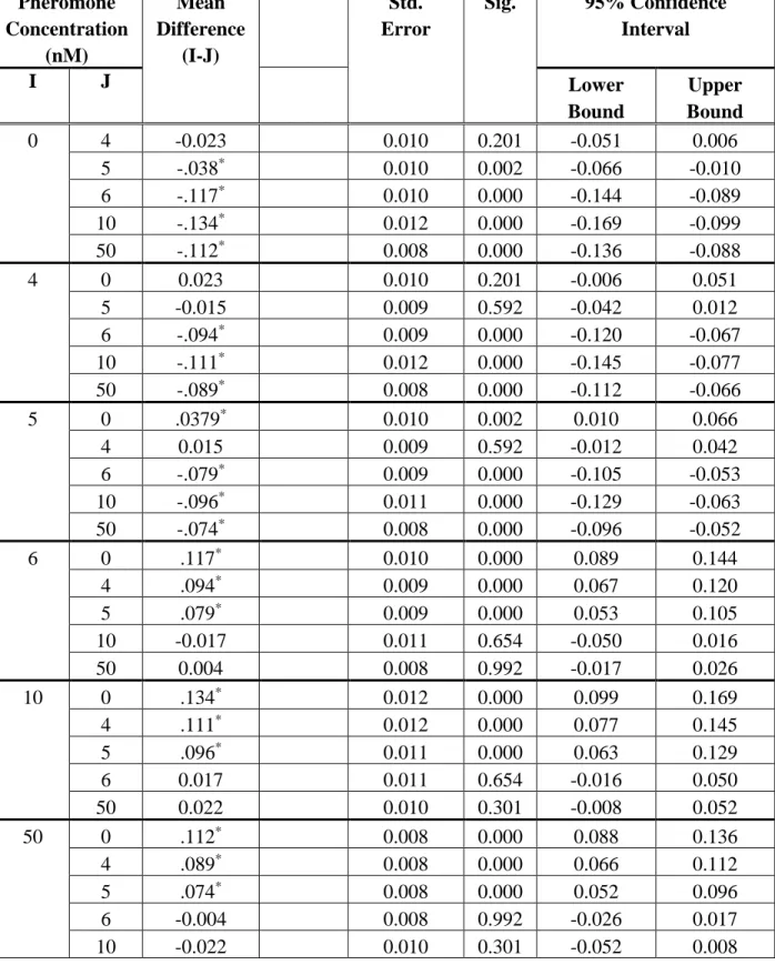
of Uniformity During Polarity Establishment... 41 Table 3.3 Games-Howell Test of Multiple Comparisons for Maximum Deviation

of Uniformity During Polarity Establishment... 42 Table 3.4 Lavene’s Test of Homogeneity of Variance for Duration of G1

Stage of the Cell Cycle During Low Pheromone Exposure ... 43 Table 3.5 Welch’s Analysis of Variance (ANOVA) for Duration of G1

Stage of the Cell Cycle During Low Pheromone Exposure ... 43 Table 3.6 Games-Howell Test of Multiple Comparisons for Duration of G1

Stage of the Cell Cycle During Low Pheromone Exposure ... 44 Table 3.7 Lavene’s Test of Homogeneity of Variance for Duration of G1 Stage

of the Cell Cycle After a One-Step Pheromone Concentration Reduction ... 50 Table 3.8 Welch’s Analysis of Variance (ANOVA) for Duration of G1 Stage

of the Cell Cycle After a One-Step Pheromone Concentration Reduction ... 50 Table 3.9 Games-Howell Test of Multiple Comparisons for Duration of G1 Stage

(13)

LIST OF FIGURES

Fig. 1.1 Dosage-Response Curves for Monostable and Bistable Models ... 5

Fig. 1.2 Budding Yeast in Different Mating States ... 7

Fig. 1.3 Pathway Diagram for the Mating Pathway... 11

Fig. 2.1 Schematic of the custom microfluidic chamber ... 25

Fig. 2.2 Segmentation process for cells ... 29

Fig. 2.3 Representative Cell Before and After Polarity Establishment and its Deviation from Uniformity ... 31

Fig. 2.4 Myo1-Ruby is an indicator of cell-cycle progression ... 34

Fig. 3.1 Cells Establish Polarity at 6 nM and Arrest Cell Cycle at 5 nM ... 39

Fig. 3.2 Polarized Cells Maintain Polarity During Multi-Step Pheromone Withdrawal ... 46

Fig. 3.3 Cells Rapidly Disassembles Polarity Upon One-Step Pheromone Reduction ... 49

Fig. 3.4 Rapid Polarity Disassembly Upon Pheromone Withdrawal is Not Due to Fluorescent Tag Disruption ... 53

Fig. 3.5 A Model of Slow-Adjusting Negative Regulation and Fast-Adjusting Positive Feedback Successfully Predicts the Influence of Initial Pheromone Concentration on Polarity Disassembly Dynamics After Pheromone Reduction ... 56

Figure 3.6 Bem3 Might Contribute to Negative Regulation of Polarity Upon One-Step Pheromone Withdrawal ... 58

(14)

xiv

LIST OF ABBREVIATIONS AND SYMBOLS

µm Micro meter

BAR Barrier

BEM Bud Emergence

bp Base pair

CDC Cell Division Cycle

CDF Cumulative Distribution Function

CLA Cln Activity dependent

DIC Differential Interference Contrast

DNA Deoxyribonucleic acid

DSE Daughter-Specific Expression

FAR Factor Arrest

FUS Cell Fusion

G protein Guanine nucleotide-binding protein

GAP GTPase Activating Protein

GDP Guanosine diphosphate

GEF Guanine nucleotide Exchange Factor

GFP Green Fluorescent Protein

GIC GTPase Interactive Components

GTP Guanosine triphosphate

Gα G protein alpha subunit

Gβ G protein beta subunit

(15)

Hrs Hours

Kb kilobase pair

Kd Dissociation Constant

KSS Kinase Suppressor of Sst2 mutations

LatA Latrunculin A

MAP Mitogen-Activated Protein

MAP2K Mitogen-activated protein kinase kinase MAP3K Mitogen-activated protein kinase kinase kinase

MAPK Mitogen-activated protein kinase

MATa Mating type a

MATα Mating type α

Myo Myosin

nM Nano mol/L

p Promoter

PAK p21-Activated Kinase

PBD Protein Binding Domain

PCR Polymerase Chain Reaction

RAC Ras-related C3 botulinum toxin substrate

RAS Rat Sarcoma

RFP Red Fluorescence Protein

RGA Rho GTPase Activating

Rho Ras Homolog family member

(16)

xvi

Sec Second

SEM Standard Error of the Mean

SKM STE20/PAK homologous Kinase related to Morphogenesis

STE Sterile

td Tandon Dimeric

yom Yeast Optimized Monomeric

YPD Yeast Extract Peptone Dextrose growth medium

(17)

CHAPTER 1 – INTRODUCTION Introduction to Polarity

In the context of cell biology, polarity establishment refers to the transition from a homogenous spatial distribution of a molecular component to an asymmetrical one. Most typically the term applies to the formation of a cell front and back or top and bottom. The

molecular components that become polarized typically include cytoskeletal proteins such as actin cables, as well as signaling molecules associated with polarity, such as Rac, Rho and Ras

proteins. Polarity establishment is required for many different physiological processes, such as cell migration, morphogenesis and differentiation. Dysregulation of polarity can often lead to diseases. For instance, polarity pathways are often perturbed by oncogenic signaling. Loss of polarity is one of the hallmarks of cancer, causing cancer cells to display alterations of cell shape, cell-cell adhesion, and cell motility. These qualities are likely important for numerous aspects of malignant transformation and play a key role in cancer metastasis (Bardwell, 2004; Iden & Collard, 2008; M. Lee & Vasioukhin, 2008)

Cell polarity often occurs in the context of gradient tracking, in which cells polarize in response to an external chemical gradient that may change in intensity, duration, or directionality over time. Polarity in response to an external cue is crucial for T-cell’s response to pathogens, fibroblast migration toward wound sites, and neuron growth toward nerve growth factor during development (Skupsky, Losert, & Nossal, 2005). Since the external cellular environment is dynamic and constantly changing, cells require regulatory mechanisms that allow them to

(18)

2

maintain a stable polarity patch while still being able to reorient their direction of polarity in response to changing environmental conditions. The signaling motifs that allow cells to adapt to changes in the cue are unknown. Elucidating and characterizing these regulatory mechanisms will have important implications for understanding complex cellular processes, such as chemotaxis and nerve growth.

Computational Models of Polarity

Various mathematical models describing polarity establishment have been proposed. A broad class of models invoke purely biochemical mechanisms that only require interactions between signaling molecules to generate spatially asymmetric concentration profiles (Causin & Facchetti, 2009; Goryachev & Pokhilko, 2008; Howell et al., 2012; Skupsky et al., 2005; Wedlich-Soldner, Altschuler, Wu, & Li, 2003). These models rely on positive feedback to amplify localized noisy regions of pathway activity and polarize through “diffusion-driven instabilities” that do not require directed transport or force generation. These models do, however, require chemical species that diffuse at different rates to keep pathway activity localized and prevent activity from spreading throughout the cell. Different diffusion rates are achieved by pathway components transitioning from the cytosol, where diffusion is fast, to the membrane, where diffusion is slow.

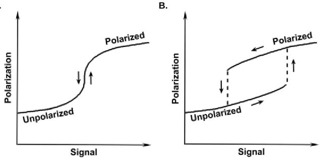
Models for diffusion-driven symmetry breaking can be further subdivided into two categories, monostable and bistable. Monostable models have one stable steady state for each stimulus level (Fig. 1.1A). Their dosage-response curves typically have a sigmoidal shape created by the positive feedback. In these models the positive feedback is sufficient to amplify the model’s response to small fluctuations in the stimulus and establish a polarize state. In contrast, in bistable models the strong positive feedback results in the existence of two stable

(19)

steady states, and cells can exist in either a polarized or unpolarized state for a range of stimulus strengths (Fig.1.1B). Bistability is a mechanism of memory, as which steady state is observed depends on past conditions. The differences between monostable and bistable models also have biological implications. Monostable models have high sensitivity, and small perturbations in stimulus can cause cells to establish or lose polarity. Therefore, monostable models can be much more reactive to changes in stimulus and allow cells to adapt to their environment quickly. Bistable models are much more robust and a larger, finite perturbation is required to initiate the polarization process. These models also feature a mechanism memory and maintain polarity against small fluctuations of stimulus once polarity is established (Ferrell, 2002; Ferrell & Xiong, 2001; Tyson, Chen, & Novak, 2003). Bistable regulation of polarity has also been suggested to improve sensitivity to shallow noisy gradients and to be the underlying mechanism behind spontaneous symmetry breaking, in which a cell polarizes in response to a spatially homogenous stimulus (Narang, 2006; Subramanian & Narang, 2004). Despite the distinct differences between models and the biological implications of favoring one model class over another, bistable or monostable regulation of polarity has not been determined experimentally.

Different models make different assumptions about the number of stable steady states the system has. Wave-Pinning models assume bistability. The solution to this model takes the form of a traveling wave, or a moving front, where the activity of the polarity protein of interest spreads like a traveling wave. The wave eventually stalls, or is pinned, due to substrate depletion of the inactive form of the molecular species. Since wave-pinning models rely on wave

propagation, these models can establish polarity at a much faster rate compared to other model designs (Mori, Jilkine, & Edelstein-Keshet, 2008; Semplice, Veglio, Naldi, Serini, & Gamba, 2012).

(20)

4

While wave-pinning models rely on bistability to establish polarity, Turing models can either be monostable or bistable. These models were first developed by the famous

mathematician Allen Turing (Turing, 1952). They rely on amplification of small local perturbations as their main polarity establishment mechanism. Turing models do not require bistability to be able to establish polarity, they can either be monostable or bistable, depending on the parameters used (Goryachev & Pokhilko, 2008; Howell et al., 2012; Onsum & Rao, 2007; Savage, Layton, & Lew, 2012). Experimentally determining whether polarity is regulated in a bistable or monostable manner will help guide future modeling efforts and give a preference to one class of models over another.

(21)

A. B.

Fig. 1.1 Dosage-Response Curves for Monostable and Bistable Models. (A) Monostable positive-feedback models have sigmoidal-shaped curves created by the strong positive feedback. (B) Bistable models have curves with two branches due to the existence of two stable steady states for a range of signal strengths. The dominance of one steady state over another depends on the history of the system, as indicated by the arrows.

(22)

6

Budding Yeast as a Model Organism for the Study of Polarity

The small Rho GTPase Cdc42 plays a central role in polarity establishment in all eukaryotic cells. Many computational models for regulation of Cdc42 polarity establishment have been proposed (Howell et al., 2012; Layton et al., 2011; Slaughter, Das, Schwartz, Rubinstein, & Li, 2009; Wedlich-Soldner et al., 2003). However, to date a systematic study to determine if the polarity circuit of any cell type is bistable has not been carried out.

Saccharomyces cerevisiae (budding yeast) is an ideal model organism for the study of polarity establishment. Budding yeast is a genetically tractable organism with relatively

well-characterized signaling pathways. At the same time, budding yeast shares many of its signaling components with other eukaryotes. Specifically, human Cdc42 can functionally substitute for its yeast counterpart, indicating that key functions of Cdc42 have been highly conserved (Shinjo et al., 1990).

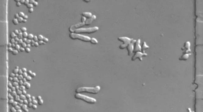
Budding yeast can exist either as a diploid or as a haploid with two mating types – a and α. Haploid cells secrete pheromone that attracts the opposite mating type and promotes cellular processes required for diploid formation. A yeast haploid cell at G1 can proceed through the cell cycle and polarize to establish a bud. Alternatively, in the presence of pheromone secreted from the opposite mating type, the cell will arrest in the G1 phase of the cell cycle and initiate the mating process. If the mating partner is nearby and high pheromone concentration is detected, the cell will form mating projections known as shmoos. If the mating partner is further away, the cell will undergo chemotropism and grow towards the potential mate, elongating into a worm-like shape (Fig. 1.2). Both budding and mating require polarity establishment to initiate the morphological changes associated with budding, shmoo-formation or chemotropism (Arkowitz, 2009; Bardwell, 2004).

(23)

Fig. 1.2 Budding Yeast in Different Mating States. BAR1 yeast cells inside our microfluidic chamber with a 0-150 nM pheromone gradient. Cells on left continue to bud, cells in center show chemotropic growth, cells on the right form mating projections.

(24)

8

The mating pathway contains a Mitogen Activated Protein Kinase (MAPK) cascade, which is the first MAPK cascade discovered. MAPK cascades are an important, well studied signaling motif that is conserved across eukaryotes. It consists of a MAP3K (in budding yeast, Ste11) that phosphorylates a MAP2K (Ste7) which phosphorylates a MAPK (Fus3), which then regulates downstream targets (Arkowitz, 2009; Bardwell, 2004). MAP kinase cascades are integral to many different types of cellular responses, such as proliferation (Geest & Coffer, 2009; Raffetto, Vasquez, Goodwin, & Menzoian, 2006; Shapiro, 2002; Zhang & Liu, 2002), differentiation (Chen, Deng, & Li, 2012; Oeztuerk-Winder & Ventura, 2012), and development (Bradham & McClay, 2006; Krens, Spaink, & Snaar-Jagalska, 2006; Oeztuerk-Winder & Ventura, 2012). These cascades often regulate polarity and cytoskeletal organization. The presence of such a well-conserved signaling cascade makes the mating pathway a great model for the study of polarity, since the results are relevant to polarity-related MAP kinase pathways in other organisms.

Budding yeast has been extensively used to study and computationally model polarity establishment in response to an internal static cue during budding (Howell et al., 2012; Layton et al., 2011; Marco, Wedlich-Soldner, Li, Altschuler, & Wu, 2007; Okada et al., 2013; Slaughter et al., 2009). Additionally, the components contributing to the positive feedback loop regulating polarity in yeast have been identified and also modeled (Bose et al., 2001; Irazoqui, Gladfelter, & Lew, 2003; Kozubowski et al., 2008; S. E. Smith et al., 2013).

Polarity establishment in yeast during mating has also been modeled recently. Several papers modeled gradient tracking and polarity reorientation in this pathway (Chou, Nie, & Yi, 2008; Dyer, Savage, Jin, & Zyla, 2013; Lakhani & Elston, 2017; McClure et al., 2015; Yi, Chen, Chou, & Nie, 2007). Since pheromone-regulated polarity in yeast is controlled by an external

(25)

stimulus that can easily be manipulated under laboratory conditions, the mating pathway of budding yeast can offer unique opportunities to experimentally study Cdc42 polarization and its role in gradient tracking. The body of computational work already done on polarity

establishment in this pathway and organism will ensure the results will be relevant for the polarity field as a whole.

Cdc42 is an Important Polarity Protein

Cdc42 is a small regulatory GTPase of the Rho family that regulates the reorganization of the actin cytoskeleton. Cdc42 also modulates other signaling pathways that induces transcription (Johnson, Jin, & Lew, 2011; Madden & Snyder, 1998). During budding, Cdc42 is initially localized to the bud site, then to the bud tip and eventually localizes to the bud neck during cytokinesis. During mating, Cdc42 is localized to the shmoo or worm tip (Richman et al., 2004). Cdc42 is essential for successful cell replication. At restrictive temperature, a temperature-sensitive mutant of Cdc42 fails to bud, and instead forms large, arrested cells (Adams, Johnson, Longnecker, Sloat, & Pringle, 1990).

Cdc42 is a GTPase, and thus acts as a molecular switch for its downstream effectors. When bound to a GTP molecule, the GTPase is in its active state and will transduce the signal to downstream effectors. However, after GTP hydrolysis, the GTPase is inactive and bound to a GDP, effectively switching the GTPase off. The GTP hydrolysis reaction is often initiated by GTPase activating proteins (GAPs) that serve as negative regulators of the pathway. GTPases are activated by Guanine nucleotide exchange factors (GEFs), which leads to the dissociation of GDP from the GTPase, allowing the GTPase to associate with a GTP molecule and become active (Rikitake & Liao, 2005). The Cdc42 GEF in budding yeast is Cdc24 (Hartwell, Mortimer, Culotti, & Culotti, 1973) and the GAPs are Bem3, Rga1 and Rga2 (Bender & Pringle, 1991;

(26)

10

Madden & Snyder, 1998; G. R. Smith, Givan, Cullen, & Sprague, 2002; Stevenson et al., 1995; Zheng et al., 1993).

The Pheromone Response Pathway and Polarity Regulation

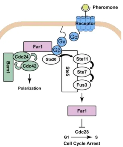
The signaling pathway for polarity establishment during mating is well-characterized (Fig. 1.3). Upon pheromone binding, the GβGγ subunits are released from the large G-protein

coupled to the pheromone receptor. The Gβ subunit triggers the MAP kinase cascade resulting in

the phosphorylation and activation of the MAP kinase Fus3. Fus3 activates transcription of pheromone-dependent genes – among them the polarity scaffold Far1. Additionally, Fus3 phosphorylates the Far1 protein, causing export of Far1 from the nucleus and protection of Far1 from degradation. Far1 inhibits the cyclin dependent kinase Cdc28, thereby arresting the cell cycle. Most significantly for polarization, Far1 forms a complex with Cdc24, the guanine nucleotide exchange factor (GEF) for Cdc42. The Far1-GEF complex is then recruited by the free Gβ subunit resulting in the activation of Cdc42 proximal to activated pheromone receptors.

Cdc42 then organizes the actin cytoskeleton and establishes polarity (Arkowitz, 2009; Bardwell, 2004).

(27)

Fig. 1.3 Pathway Diagram for the Mating Pathway. Receptor and its coupled G protein are shown in blue. Components of the positive feedback regulating polarity shown in green.

(28)

12

The mating pathway has a well-characterized polarity positive feedback loop, mediated by a complex comprised of the Cdc42 GEF, Cdc24, and the scaffold, Bem1, which binds to active Cdc42. Activated Cdc42 recruits the Bem1-GEF complex, which in turn catalyzes the activation of more Cdc42. This results in robust positive feedback that can amplify a shallow, noisy stimulus gradient to maximal pathway activation (Bose et al., 2001; Irazoqui et al., 2003; Kozubowski et al., 2008; S. E. Smith et al., 2013).

Here we use the pheromone response pathway to show that Cdc42 polarity establishment is a bistable process that shows hysteresis. Unpolarized cells require 6 nM pheromone to

establish polarity. In contrast, cells that established polarity in a high pheromone concentration will remain polarized through a multi-step reduction of pheromone concentration to 0 nM. Additionally, we demonstrate that polarized cells will lose their polarity if pheromone is sufficiently reduced in a one-step fashion. These results suggest a model of a positive feedback that adjusts to changes in pheromone concentration quickly, combined with a negative feedback that adjusts slowly. The model predicts that the pheromone concentration prior to a one-step decrease will determine whether cells will maintain or disassemble polarity, and at which rate. We show that these predictions hold experimentally, thus confirming the model.

(29)

CHAPTER 2 - MATERIALS AND METHODS Experimental Design

To determine whether polarity establishment is a monostable or bistable process, we employed an approach integrating traditional yeast genetics and cutting-edge microfluidics-enabled microscopy with computational image analysis to resolve signaling mechanisms occurring at different time scales and provide a quantitative understanding of dynamic cell polarity. We first constructed a strain containing the polarity scaffold protein Bem1 tagged with yomNeonGreen fluorescent tag. The strain also contained a deletion of the BAR1 gene coding for a protease that degrades pheromone (Barkai, Rose, & Wingreen, 1998; Ciejek & Thorner, 1979; Sprague & Herskowitz, 1981). Lastly, the strain also contained the myosin II light-chain Myo1 tagged with yomRuby red fluorescent protein. Since Myo1 localizes to the bud neck in all stages of the cell cycle with the exception of G1, the tag will allow us to exclude from our analysis cells that are going through the budding cycle (Fig. 2.4). We then employed a series of microfluidic microscopy experiments followed by rigorous image analysis to quantify the data and determine whether Cdc42 polarity is monostable or bistable. Following is a detailed description of the methods we employed.

Yeast Strains and Genetic Procedures

Table 2.1 lists yeast strains used in these studies. Table 2.2 lists the sequence of oligonucleotides used for PCR fragment amplification, mutagenesis, and DNA sequence

(30)

14

genetic methods for transformation, gene replacement, crosses, and tetrad dissection were as described in Amberg et al.(2005).

(31)

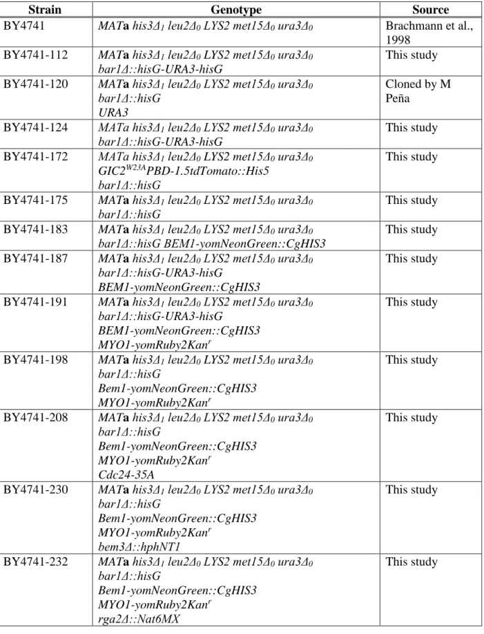
Table 2.1 Budding Yeast Strains Constructed in this Study

Strain Genotype Source

BY4741 MATa his3Δ1 leu2Δ0 LYS2 met15Δ0 ura3Δ0 Brachmann et al.,

1998 BY4741-112 MATa his3Δ1 leu2Δ0 LYS2 met15Δ0 ura3Δ0

bar1Δ::hisG-URA3-hisG

This study BY4741-120 MATa his3Δ1 leu2Δ0 LYS2 met15Δ0 ura3Δ0

bar1Δ::hisG URA3

Cloned by M Peña

BY4741-124 MATa his3Δ1 leu2Δ0 LYS2 met15Δ0 ura3Δ0 bar1Δ::hisG-URA3-hisG

This study BY4741-172 MATa his3Δ1 leu2Δ0 LYS2 met15Δ0 ura3Δ0

GIC2W23APBD-1.5tdTomato::His5 bar1Δ::hisG

This study

BY4741-175 MATa his3Δ1 leu2Δ0 LYS2 met15Δ0 ura3Δ0 bar1Δ::hisG

bar1Δ::hisG BEM1-yomNeonGreen::CgHIS3

bar1Δ::hisG-URA3-hisG

BEM1-yomNeonGreen::CgHIS3

This study

BY4741-191 MATa his3Δ1 leu2Δ0 LYS2 met15Δ0 ura3Δ0 bar1Δ::hisG-URA3-hisG

BEM1-yomNeonGreen::CgHIS3 MYO1-yomRuby2Kanr

This study

Bem1-yomNeonGreen::CgHIS3 MYO1-yomRuby2Kanr

This study

Cdc24-35A

This study

bem3Δ::hphNT1

This study

rga2Δ::Nat6MX

(32)

16

rga1Δ::hphNT1

This study

BY4742 MATα his3Δ1 leu2Δ0 lys2Δ0 MET15 ura3Δ0 Brachmann et al.,

1998 BY4742-32 MATα his3Δ1 leu2Δ0 lys2Δ0 MET15 ura3Δ0

bar1Δ::hisG-URA3-hisG This study

BY4742-51 MATα his3Δ1 leu2Δ0 lys2Δ0 MET15 ura3Δ0 bar1Δ::hisG

BEM1-yomNeonGreen::CgHIS3

This study

BY4742-56 MATα his3Δ1 leu2Δ0 lys2Δ0 MET15 ura3Δ0 bar1Δ::hisG

BEM1-yomNeonGreen::CgHIS3 MYO1-yomRuby2Kanr

(33)

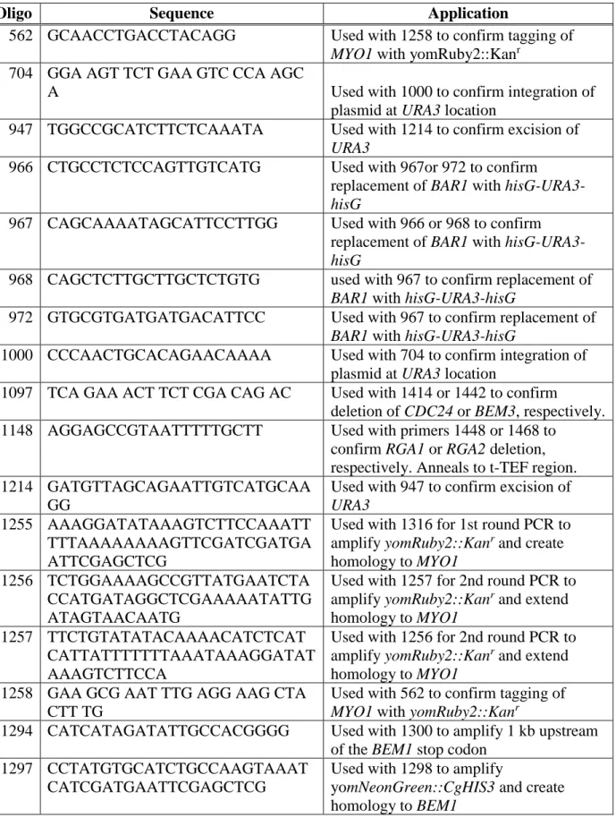
Table 2.2 Oligonucleotides Used in this Study

Oligo Sequence Application

562 GCAACCTGACCTACAGG Used with 1258 to confirm tagging of

MYO1 with yomRuby2::Kanr

704 GGA AGT TCT GAA GTC CCA AGC

A Used with 1000 to confirm integration of

plasmid at URA3 location

947 TGGCCGCATCTTCTCAAATA Used with 1214 to confirm excision of

URA3

966 CTGCCTCTCCAGTTGTCATG Used with 967or 972 to confirm

replacement of BAR1 with

hisG-URA3-hisG

967 CAGCAAAATAGCATTCCTTGG Used with 966 or 968 to confirm

replacement of BAR1 with

hisG-URA3-hisG

968 CAGCTCTTGCTTGCTCTGTG used with 967 to confirm replacement of

BAR1 with hisG-URA3-hisG

972 GTGCGTGATGATGACATTCC Used with 967 to confirm replacement of

BAR1 with hisG-URA3-hisG

1000 CCCAACTGCACAGAACAAAA Used with 704 to confirm integration of

plasmid at URA3 location

1097 TCA GAA ACT TCT CGA CAG AC Used with 1414 or 1442 to confirm

deletion of CDC24 or BEM3, respectively.

1148 AGGAGCCGTAATTTTTGCTT Used with primers 1448 or 1468 to

confirm RGA1 or RGA2 deletion, respectively. Anneals to t-TEF region. 1214 GATGTTAGCAGAATTGTCATGCAA

GG

Used with 947 to confirm excision of

URA3

1255 AAAGGATATAAAGTCTTCCAAATT TTTAAAAAAAAGTTCGATCGATGA ATTCGAGCTCG

Used with 1316 for 1st round PCR to amplify yomRuby2::Kanr and create homology to MYO1

1256 TCTGGAAAAGCCGTTATGAATCTA CCATGATAGGCTCGAAAAATATTG ATAGTAACAATG

Used with 1257 for 2nd round PCR to amplify yomRuby2::Kanr and extend homology to MYO1

1257 TTCTGTATATACAAAACATCTCAT CATTATTTTTTTAAATAAAGGATAT AAAGTCTTCCA

Used with 1256 for 2nd round PCR to amplify yomRuby2::Kanr and extend homology to MYO1

1258 GAA GCG AAT TTG AGG AAG CTA CTT TG

Used with 562 to confirm tagging of

MYO1 with yomRuby2::Kanr

1294 CATCATAGATATTGCCACGGGG Used with 1300 to amplify 1 kb upstream

of the BEM1 stop codon 1297 CCTATGTGCATCTGCCAAGTAAAT

CATCGATGAATTCGAGCTCG

Used with 1298 to amplify

yomNeonGreen::CgHIS3 and create homology to BEM1

(34)

18 1298 CGAGCTCGAATTCATCGATGATTT

ACTTGGCAGATGCACATAGG

Used with 1297 to amplify

yomNeonGreen::CgHIS3 and create homology to BEM1

1299 AGGGACTCACATCTATCTTGGG Used with 1301 to amplify 1 kb

downstream of the BEM1 stop codon 1300 GGCTTGGATTATGTTACTGACTTGT

G

Used with 1294 to amplify 1 kb upstream of the BEM1 stop codon

1301 TTACTTGGCAGATGCACATAGG Used with 1299 to amplify 1 kb

downstream of the BEM1 stop codon 1316 AAATATTGATAGTAACAATGCACA

GAGTAAAATTTTCAGTGGTGCTGG TTTAATTAAC

Used with 1255 for 1st round PCR to amplify yomRuby2::Kanr and create homology to MYO1

1354 AATTGGTCGACTTGGAGGGC Used with 1360 to confirm tagging of

BEM1 with yomNeonGreen::CgHIS3

1360 CCAGCACCAGCACCTGC Used with 1354 to confirm tagging of

BEM1 with yomNeonGreen::CgHIS3

1414 GCAGAAGAGTACCATTGCTGTTAT C

Used with 1097 to confirm replacement of

CDC24 with pCORE-UK

1426 TCCAACCCGAGAGATCATGGCGAT CCAAACCCGTTTTGCCCCGCGCGT TGGCCGATTCAT

Used with 1427 to amplify pCORE-UK and create homology to 2999 bp in

CDC24

1427 AATCCCCATCTTCGTCCTGATATTT GATCTTGGTGATTGGTTCGTACGC TGCAGGTCGAC

Used with 1426 to amplify pCORE-UK and create homology to 2999 bp in

CDC24

1430

CCCCTGTTGGTCAAAGAATTGC

Used with 1431 to amplify a 1kb fragment that could be cut with PstI to screen for

CDC24-35A transformants

1431

GCGGCTGTTGTGATGATTCG

Used with 1430 to amplify a 1kb fragment that could be cut with PstI to screen for

CDC24-35A transformants

1432

TGTTGCCTAGCCCTATCAAGACC Used with 1433 to amplify cdc24-35A for

TOPO cloning and sequencing 1433

CAAAATCCCCATCTTCGTCCTG Used with 1432 to amplify cdc24-35A for

TOPO cloning and sequencing 1434

CTAACCGGGACGCTGCTGAC

Second primer used to sequence Cdc24-35A (first primer is the TOPO m-13 reverse primer)

1435 GACGCGTGGTCAACTGGAAG Third primer used to sequence Cdc24-35A

1436 CCGCAAAACAACCGGTCA Forth primer used to sequence Cdc24-35A

1438 GCCTTTTGTTCGAGTTCGTGATTAC ATCAGGCATATACAAGGTCGACGG ATCCCCGGG

Used with 1439 for 1st round PCR to amplify a pFA6 plasmid and create homology to BEM3

1439 ATGGAGGTTTACTGGCAACGTTAT ATTTCTACAATTTTAGATCGATGA ATTCGAGCTCG

Used with 1438 for 1st round PCR to amplify a pFA6 plasmid and create homology to BEM3

(35)

1440 TTTTTCTCTTTTCTTCTTTGTCCTTG CCTTCTACCATTTTGCCTTTTGTTC GAGTTCGTG

Used with 1441 for 2nd round PCR to amplify a pFA6 plasmid and extend homology to BEM3

1441 AAGCCTCTATACATCTCGCCCTCTT TCTATCATTAAATCAATGGAGGTT TACTGGCAACG

Used with 1440 for 2nd round PCR to amplify a pFA6 plasmid and extend homology to BEM3

1442 CGGCGGTGATGTTGGAAAAA Used with 1097 to confirm deletion of

BEM3

1444 AGCTGATTCAGGTACTAGTGGTGG

AGAGAGCGGCATATTAAAGGTCG ACGGATCCCCGGG

Used with 1445 for 1st round PCR to amplify pFA6 plasmid and create homology to RGA1

1445 CAGTTCATATAAGGCGGCTCAATG

CAGAACCGAGGATAGCGATCGAT GAATTCGAGCTCG

1446 ACATTTATCTCTATTATAGCTTTTT GTACAAGACAAGGATAGCTGATTC AGGTACTAGTG

Used with 1447 for 2nd round PCR to amplify pFA6 plasmid and extend homology to RGA1

1447 CCTGCTTAAGTCTGCGATTAAAAA AATAACGTTTCGATACAGTTCATA TAAGGCGGCTCA

1448 CAAAATACCGAAACGCCAAA Used with primer 1148 to confirm RGA1

deletion 1467 ACTATTTTCTTACTTTATTCTTTTTT

CATATGATTTCTTATTTAATCTATC CTATGTTTA

1468 GGCAAGTTTGACGTTCACTG Used with primer 1148 to confirm RGA2

replacement with a pFA6 plasmid 1475 AACGTAGCATCTCAAGAGCAAGG

AGATTTTGATGAAAAAAATGGTCG ACGGATCCCCGGG

1476 TTTAATCTATCCTATGTTTATTTAA CTTTTGCAAATCTGTAATCGATGA ATTCGAGCTCG

1477 ATTACCAAGAGTTCATTGTACTTTT AATAAAGTGAAATATAACGTAGCA TCTCAAGAGCA

Used with 1467 for 2nd_{round PCR to}

amplify pFA6 plasmid and extend homology to RGA2

(36)

20

The bar1Δ strain BY4741-112 was constructed from BY4741 using the one-step gene replacement method (Rothstein, 1983) to replace the BAR1 locus. The replacement used the EcoRI–SalI fragment from pJGsst1 (Reneke, Blumer, Courchesne, & Thorner, 1988) that carries the bar1Δ::hisG-URA3-hisG allele. Transformants were isolated using –Ura synthetic media plates. Replacement of the BAR1 locus was confirmed with colony PCR analysis using yeast genomic DNA as template with primer pairs 967/968, 972/966 and 967/966. Strains BY4741-124 and BY4742-32 are segregants resulting from the cross of BY4741-112 and BY4742. Strain BY4741-175 was generated from the BY4741-124 strain by selection on 5-fluoroorotic acid (Life Technologies, Grand Island, NY) medium (Boeke, LaCroute, & Fink, 1984). This medium provides a positive selection for isolates in which the URA3 marker is excised by recombination within the direct hisG repeats (Alani, Cao, & Kleckner, 1987). Successful excision was confirmed with colony PCR analysis using yeast genomic DNA as template with primers pairs 972/968 and 1214/947.

The GIC2W23APBD-1.5tdTomato::His5 strain BY4741-172 was constructed from

BY4741-120 also using the integrative plasmid YIp211-GIC2PBD-RFP (Tong et al., 2007) that was cut with the ApaI restriction enzyme (New England Biolabs, Ipswich, MA). Successful integration was confirmed with colony PCR analysis using yeast genomic DNA as a template with primers 1000/704.

The BEM1-yomNeonGreen strain BY4741-183 was constructed as follows. Plasmid pDML99 (Landgraf, Huh, Hallacli, & Lindquist, 2016) was used as a template for a PCR reaction with primer pair 1297/1298. Genomic DNA from strain BY4741-175 was used as a template for two PCR reactions to generate homology to 1kb downstream and 1kb upstream of the BEM1 stop codon using primer pairs 1299/1301, and 1300/1294, respectively. The three PCR

(37)

products were assembled using Gibson Assembly (New England Biolabs, Ipswich, MA), and the resulting product was used for transformation of BY4741-175. Transformants were selected on – His synthetic media plates. The integration of yomNeonGreen at BEM1 was confirmed with colony PCR analysis using yeast genomic DNA as template with primer pair 1354/ 1360. Strains BY4741-187 and BY4742-51 are segregants of a cross between BY4141-183 and BY4742-32. To confirm that the BEM1-yomNeonGreen fusion strain responded normally to pheromone, the morphology of BY4741-187 and BY4741-175 cells responding to 0 nM, 10 nM and 50 nM pheromone was compared. For this comparison, cells from the parallel cultures were fixed with 2% formaldehyde at 0, 2 and 5.5 hrs. The vegetative, chemotropic or mating competent

morphology of the fixed cells was scored and quantified using a hemocytometer.

The BEM1-yomNeonGreen MYO1-yomRuby2 strain BY4141-191 was created by transforming strain BY4741-187 with the MYO1-yomRuby2-Kanr allele. Plasmid pFA6a-link-yomRuby2-Kanr_{(S. Lee, Lim, & Thorn, 2013) was used a template for a first round PCR}

reaction with primer pair 1316/1255. The product of this reaction was used as a template for a second PCR reaction with primer pair 1256/1257. The resulting product was used for

transformation of BY4741-187. Transformants were selected on complete media plates containing G418 (Sigma-Aldrich, St. Louis MO). Integration of yomRuby2 at the MYO1 locus was confirmed by colony PCR analysis using yeast genomic DNA as template with primer pair 1258/562. Strains BY4741-198 and BY4742-56 are segregants of a cross between BY4741-191 and BY4742-51. To confirm that BY4741-198 responded normally to pheromone, the

morphology of cells exposed to pheromone was compared to that of BY4741-175 in the procedure described above except that cells were fixed at 0, 2 and 4 hrs.

(38)

22

The unphosphorylatable CDC24-35A mutant strain BY4741-208 was created by a serial transformation of a diploid resulting from a cross of strains BY4741-198 and BY4742-56. Because CDC24 is an essential gene the transformation could only be done in a diploid containing two copies of CDC24. The first step was a transformation of the diploid with a

cdc24Δ::CORE-UH allele that was generated in a PCR reaction using the pCORE-UH plasmid

(Storici & Resnick, 2006) as a template with primers 1426/1427. Deletion of one of the copies of CDC24 was confirmed by colony PCR analysis using yeast genomic DNA as template with primer pair 1414 and 1097. Plasmid pSW86 (Wai, Gerber, & Li, 2009) was digested with the restriction enzymes HindIII and HpaI (New England Biolabs, Ipswich, MA), and the resulting 2999 bp fragment was used to replace the cdc24Δ::CORE-UH allele. The transformation was confirmed with colony PCR analysis using yeast genomic DNA as template with primer pair 1430/1431 and a subsequent digestion of the product using the PstI restriction enzyme (New England Biolabs, Ipswich, MA). The diploid was then sporulated and subjected to tetrad analysis for the recovery of haploid segregants. Haploids containing the CDC24-35A allele were

identified using the PstI restriction strategy described above. A DNA fragment from all segregants of interest was amplified with colony PCR using yeast genomic DNA as template with primer pair 1432/1433. The amplified fragment from each segregant was cloned into the pCR Blunt II Topo vector (Invitrogen Life Technologies, Grand Island, NY) and sequenced using M13R, 1434, 1435 and 1436 primers to ensure the presence of all mutation sites using the University of North Carolina – Chapel Hill Core Facilities.

The bem3Δ::hphNT1 strain 230 was created by transforming strain BY4741-198. Plasmid pFA6a-hphNT1 (Hentges, Van Driessche, Tafforeau, Vandenhaute, & Carr, 2005) was used a template for a first round PCR reaction with primer pair 1438/1439. The product of

(39)

this reaction was used as a template for a second PCR reaction with primer pair 1440/1441. The resulting product was used for transformation of BY4741-198. Transformants were selected on complete media plates containing Hygromycin B (Sigma-Aldrich, St. Louis MO). Deletion of

BEM3 was confirmed by colony PCR analysis using yeast genomic DNA as template with

primer pair 1441/1097.

The rga2Δ::Nat6MX strain BY4741-232 was also created by transforming strain BY4741-198. Plasmid pFA6a-Nat6MX (Hentges et al., 2005) was used a template for a first round PCR reaction with primer pair 1475/1476. The product of this reaction was used as a template for a second PCR reaction with primer pair 1477/1467. The resulting product was used for transformation of BY4741-198. Transformants were selected on complete media plates containing Nourseothricin (Sigma-Aldrich, St. Louis MO). Deletion of RGA2 was confirmed by colony PCR analysis using yeast genomic DNA as template with primer pair 1468/1148.

The rga1Δ::HphNT1 strain 234 was created by transforming strain BY4741-198. Plasmid pFA6a-hphNT1 (Hentges et al., 2005) was used a template for a first round PCR reaction with primer pair 1444/1445. The product of this reaction was used as a template for a second PCR reaction with primer pair 1446/1447. The resulting product was used for

transformation of BY4741-198. Transformants were selected on complete media plates

containing Hygromycin B (Sigma-Aldrich, St. Louis MO). Deletion of RGA1 was confirmed by colony PCR analysis using yeast genomic DNA as template with primer pair 1448/1097.

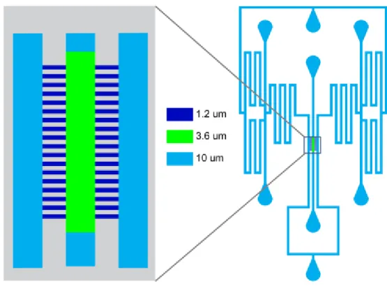
Microfluidic Technology to Image Cell Response with a Fast Time-Resolution

The microfluidic device used has a simple design featuring four inputs, two at each side of the chamber, and four outputs located along the center of the device (Fig. 2.1). In the center of the device is a main chamber with a ceiling height of 3.6 µm, which is the area of the device

(40)

24

containing cells to be imaged. Two feeding channels flow on both sides and connect to the main chamber with microchannels that are 1.2 µm tall. The rest of the channels in the device are 10 µm tall. Cells are loaded into the device through the two middle output channels. The shorter ceiling in the main chamber causes the cells to stop their flow and remain stationary, while the microchannels feed media into the main chamber and replenish nutrients and pheromone. Once cell loading is complete, all output channels are used to collect excess media coming in from the input syringes, the feeding channels and the main chamber. A new chamber was used for every experiment. All chambers for this project were poured off of the same mold to ensure

consistency among experiments and reduce error.

The two input ports on each side of the chamber are connected to syringes containing different concentrations of pheromone (or no pheromone at all). Changing the relative heights of the input syringes can change the concentration of pheromone flowing into the main chamber where the cells reside. The syringe heights can be manipulated so the cells see the pheromone concentration contained by either one of the syringes, or an intermediate pheromone

concentration. The long and curvy features of the feeding channels ensure an intermediate pheromone concentration will be well-mixed before flowing into the main chamber. The height of the syringes was changed by an automatic robot built according to instructions from the Hasty lab Dial-A-Wave motor with hardware version 2 configuration (Ferry, Razinkov, & Hasty, 2011).

(41)

Fig. 2.1 Schematic of the custom microfluidic chamber. On left, enlargement of main chamber. Cell loading zone is in green and microchannels are in royal blue.

(42)

26

Using the microfluidic device allows quick pheromone concentration changes. The pheromone concentration within the main chamber changes within ̴10 sec of syringe height adjustment. The innovative experimental design results in single-cell quantitative data with the short time resolution needed to characterize cell response in real time.

Time-lapse imaging to follow pheromone-regulated polarity, morphology and cell cycle arrest

The experiments were done in microfluidic device and cell culturing methods as

described in the supplement to Hao et al., 2008. An overnight cell culture was grown in synthetic complete medium. In the morning of the experiments, the culture was diluted and incubated for two doubling times. Prior to loading cells into the chamber, cells were counted and budding index was calculated to ensure the culture was in early log phase (0.5-1x107 cells/mL). The culture was then diluted to a cell density of 1-2x106 cells/mL to optimize loading into the chamber and ensure consistent experimental conditions.

Alexa 647 (Thermo Fisher Scientific, Waltham, Massachusetts, USA) dye was added to pheromone containing media to track changes in pheromone concentrations throughout the experiment. Images of the dye at both junctions leading to the chamber were acquired and syringe positions were adjusted to ensure that pheromone flow would match from both sides of the chamber. Images of the dye in the main chamber were acquired during experimental set up to construct a calibration curve for the motor controlling the syringes. The chamber was imaged to ensure dye turned on and off within less than 20 seconds.

Microscopy was performed with an Olympus IX81 motorized inverted confocal spinning disk microscope using a Plan Apo N 60×/1.42 oil objective and a iXon ultra EMCCD camera. Acquisition was performed with MetaMorph software (Molecular Devices, Sunnyvale, CA). The 488 nm laser was set to 2% intensity, the 561 nm laser to 6% intensity, the 640 nm laser to 5%

(43)

intensity and the 450 nm laser to 0% intensity. GFP (488 nM) and differential interference contrast images of cells from seven different stage positions were taken every 5-minutes. RFP (651 nM) images were taken every 10 minutes and the dye (640 nM) was imaged every 25 minutes. In experiments where pheromone concentration was switched from a higher concentration (50 nM or 10 nM) to a lower concentration (0-6 nM) in one step, higher acquisition rates were used around the transition point. DIC and GFP images were acquired every 2.5 minutes starting 10 minutes prior to the concentration change and ending 30 minutes after the change. The acquisition interval for all other wavelengths was unchanged.

Cell segmentation and quantification of cell polarity

Image processing and cell scoring were aided by use of ImageJ software (Schneider, Rasband, & Eliceiri, 2012). A Gaussian filter with sigma of 1 was applied to the Images for all fluorescence channels to get rid of camera-related noise. A z projection of max intensity was used for all z stacks and a background subtraction with a radius of 50 was applied. Images were registered using the Descriptor Based Series Registration plugin. Registration for all channels was done based on the model found for the DIC series.

Inner boundaries between cells close to one another were extracted from the DIC series using the edge-detection function in MatLab (The MathWorks, 2015). Edges were detected using two different thresholds with the Sobel method. The less refined edges were then filled and eroded to create a mask that was smaller than the surface of the cells themselves. The eroded mask was used to multiply the refined edges detected using the algorithm, creating a mask that retained only the inner boundaries between cells and omitting the boundaries between cells and their environment.

(44)

28

The edge detection function was applied to the original DIC series again using the Sobel edge detection method with a coarse threshold. The edges were dilated, closed and filled in order to create a mask that was much larger than the cells themselves, minimize the areas of the images treated by the cell segmentation algorithm and speed up the data analysis process. Both masks (the inner boundary mask and the larger mask) were manually checked to ensure they correctly represented boundaries between cells and corrected when necessary. The two masks were then applied to the GFP images using a simple image multiplication in ImageJ.

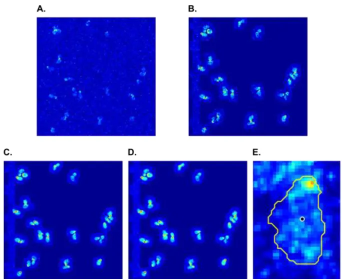
Cells were then segmented using SegmentMe_2D (Fig. 2.2) (Tsygankov, Chu, Chen, Elston, & Hahn, 2014). The masked GFP movies were loaded to Segment Me. A dynamic filter was applied by averaging every image with the time points that preceded and followed it. An additional Gaussian filter of a size 15 and a σ=1 was applied to the images. Water shedding was then applied to the images using 45 different thresholds. After examination of the segmentation results, the single, most successful, threshold was chosen and used to segment the cells. The cells were then tracked through time in order to generate a single time series for every cell.

(45)

Fig. 2.2 Segmentation process for cells. (A) Raw GFP images (B) Image with DIC mask applied. (C) Image with dynamic filter applied (D) Image with Gaussian filter applied. (E) Single-cell raw data with the final segmentation mask applied in yellow.

(46)

30

Once the cells were segmented and tracked, the final masks were applied to the original registered background-subtracted GFP z-projection. The original data was quantified for each cell using SegmentMe_2D. Only cells that were determined to be in G1 by the absence of a visible Myo1-yomRuby spot at the beginning of the relevant time span were analyzed (Fig. 2.4). Single cell data was truncated when cells entered S phase of the cell cycle, as determined by the appearance of a visible Myo1 spot, and these cells were dropped from the mean for the following time points.

Different data quantification methods were compared to identify the most appropriate one. Methods that were examined included area of the polarity patch, mean intensity per pixel, total intensity of the cell, coefficient of variation of pixel intensity and deviation from

uniformity. The method of deviation from uniformity was chosen, since it was the least sensitive to changes in total polarity protein expression, changes in cell size and changes in illumination conditions from one experiment to another. The method was also the most sensitive to changes in polarity protein distribution and captured small noisy fluctuations in polarity patch stability. Therefore, this method was the most sensitive to distribution changes while being the least sensitive to other variations between cells and experiments.

(47)

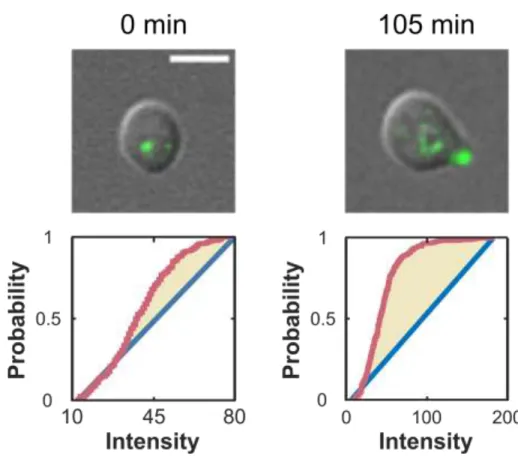
Fig. 2.3 Representative Cell Before and After Polarity Establishment and its Deviation from Uniformity. The upper panel shows a representative cell that was exposed to 50 nM pheromone and is shown at 0 min and at 105 min, after a tight polarity patch has been established. Bottom panels show the calculation of deviation from uniformity for both time points. Pink curves are the experimental CDF for pixel intensity. Blue curves are the CDF of an equivalent homogeneous distribution. The tan area between the curve is the integral on which the deviation from uniformity is based. At 0 min the cell has a deviation from uniformity of 0.209, and at 105 min one of 0.546.

(48)

32

Deviation from uniformity for fluorescence of the polarity marker

(Bem1-yomNeonGreen) was calculated for each cell at each time point (Fig. 2.3) in SegmentMe_2D based on the Kolmogorov-Smirnov test to compare the experimental pixel distribution to an equivalent uniform homogenous distribution (Justel, Pefia, & Zamar, 1997; Tsygankov et al., 2014). For each segmented cell, at each time point, the highest (Imax) and lowest intensity (Imin)

values were determined. A homogeneous uniform distribution was generated between these two values. The cumulative distribution function was calculated for the homogenous uniform

distribution as well as the experimental pixel intensity distribution. The integral between the two cumulative distribution functions was taken and normalized to be a value between 0 and 1.

The procedure is captured in the following equations: For a single segmented cell in a single time point, 𝐼_𝑖,𝑗

𝐼𝑚𝑖𝑛= min_𝑖,𝑗 𝐼𝑖,𝑗 𝐼_𝑚𝑎𝑥 = max 𝑖.𝑗 𝐼𝑖,𝑗 𝑥_𝑛 = 𝐼_𝑚𝑖𝑛+ 𝑛 − 1 𝑁 − 1(𝐼𝑚𝑎𝑥− 𝐼𝑚𝑖𝑛) where 𝑛 = 1,2, … , 𝑁 𝑖 = 1,2, … . , 𝐼 and 𝑗 = 1,2, … , 𝐽.

The cumulative intensity distribution is

𝑦_𝑛 =_𝐼𝐽1 ∑ 𝐻(𝐼_𝑖,𝑗 _𝑖,𝑗, 𝑥_𝑛) where 𝐻(𝐼𝑖,𝑗, 𝑥𝑛) = {

1 𝑖𝑓 𝐼𝑖,𝑗< 𝑥𝑛

0 𝑖𝑓 𝐼_𝑖,𝑗≥ 𝑥_𝑛

For a uniform homogenous distribution, the cumulative distribution is: 𝑈_𝑛 ≈ 𝑥𝑛 − 𝐼𝑚𝑖𝑛

𝐼_𝑚𝑎𝑥− 𝐼_𝑚𝑖𝑛= 𝑛 − 1 𝑁 − 1 The deviation from uniformity is:

(49)

𝑃 = 2

𝑁∑(𝑦𝑛− 𝑈𝑛)

𝑁 𝑛=1

𝑦𝑛 ∈ [0,1], 𝑃 ∈ [0,1]

The mean of the deviation from uniformity for all cells was taken and the standard error calculated for each time point. The mean +/- standard error were plotted in Matlab (The MathWorks, 2015).

To determine the maximum deviation from uniformity cells achieved while in the G1 stage of the cell cycle, each single cell time trace was smoothed in Matlab (The MathWorks, 2015) using a 3 time point averaging window, and the trace was truncated either when the cell entered S-phase or after 2 hrs., whichever came first. The maximum value for each smoothed single cell trace was determined in Matlab and the results were plotted as a box and whiskers plot.

Identification and quantification of G1 cells

Myo1 is a myosin II subunit that is required for actomyosin contractile ring contraction and cell separation after cytokinesis. Myo1 localizes to the bud neck between the S-phase of the cell cycle and the completion of cytokinesis and is visible by microscopy in all stages of the cell cycle but G1. The length of time each cell remained in the G1 phase of the cell cycle was determined by eye based on the appearance of a Myo1-yomRuby spot when a cell entered the S-phase of the cell cycle. The results were plotted as a box and whiskers plot in Matlab (The MathWorks, 2015). The percent of cells in the G1 phase of the cell cycle was determined for each replica of the experiment. The results for the three replicas were averaged for each time point and the standard error was calculated. The mean +/- standard error were plotted in Matlab.

(50)

34

Fig. 2.4 Myo1-Ruby is an indicator of cell-cycle progression. Panel shows a representative cell that was imaged in the absence of pheromone in a microfluidic chamber. Myo1 clearly localizes to the bud neck in all stages of the cell cycle with the exception of G1. The points of cell cycle entry and exit are indicated by a white arrow pointing to Myo1 localization.

(51)

Statistical analysis was used to determine statistically significant differences between different dosages’ maximum deviation from uniformity and length of time cells spent in G1. First, a Levene Absolute multiple-sample test for equal variance was used in Matlab to determine if the homogeneity of variance assumption was violated. Since all data sets violated the

assumption, a Welch F test was run using IBM SPSS. Since the test showed significant differences for all data, a Games-Howell post hoc test in IBM SPSS was used to determine which data sets are significantly different from each other (IBM Corp., 2011).

(52)

36

CHAPTER 3 – RESULTS Polarity Establishment Requires 6 nM Pheromone

One of the hallmark features of a bistable system is hysteresis. Hysteresis refers to a mechanism of memory in which the observed response of a system depends on its history (Fig. 1.1). Therefore, we designed experiments to look for hysteretic behavior in pheromone-regulated polarity. In particular, we asked if the minimum pheromone concentration required to establish polarity is greater than the minimum pheromone concentration required to maintain an existing polarity patch. To answer this question, we used live-cell imaging performed in microfluidic chambers designed to allow precise temporal control of pheromone concentration. To visualize polarity assembly and disassembly, we tagged the scaffold protein Bem1 with a yomNeonGreen fluorescent tag. To quantify the degree to which individual cells polarize, we calculated the deviation from uniformity for fluorescently tagged Bem1. The deviation from uniformity

measures the amount that the experimentally determined fluorescence distribution within a single cell deviates from a uniform distribution at a given time point (Fig. 2.3).

Cells can establish polarity through either the pheromone pathway during the G1 phase of the cell cycle, or as part of the cell cycle during the G1 to S phase transition. To ensure that only cells that polarized in response to pheromone were included in our analysis, we tagged the Myo1 subunit of Myosin II with a yomRuby2 fluorescent tag. Myo1 localizes to the bud neck during all stages of the cell cycle except G1 (Fig. 2.4). Therefore, our analysis only included unbudded cells lacking localized Myo1.

(53)

We first determined the minimum pheromone concentration required for naïve cells to polarize. To make this determination, we monitored polarity establishment for cells exposed to six pheromone concentrations (Fig. 3.1A-C). Cells in the G1 stage of the cell cycle exposed to 0 nM and 4 nM responded similarly and failed to polarize before progressing through the cell cycle. At 5 nM, cells showed a heterogeneous response, with some cells establishing a weak polarity patch, while others remained unpolarized. The cells that established polarity showed a very unstable polarity patch that appeared and disappeared throughout the experiment. At 6 nM the majority of cells established a weak yet stable polarity patch, but the polarization process was slow (~80 mins). Polarity establishment proceeded in a similar fashion at 10 and 50 nM.

However, at these high concentrations of pheromone cells established polarity more quickly (~40 min) and in a switch-like manner. One possible explanation for the difference in the polarization rate between 6 nM and the higher doses, is that 6 nM is near the transition point, close to the sigmoidal slope or close to where the polarity circuit switches from a bistable to a monostable system (Fig. 3.1A and B, respectively), and molecular-level fluctuations are required to activate the positive feedback and establish polarity. At higher doses that are further from the transition point, the positive feedback is activated much faster without relying on fluctuations. At all doses, there was a ~20 min delay before cells began to establish polarity, suggesting that polarity requires the accumulation of one or more pathway components.

(54)

(55)

Fig. 3.1 Cells Establish Polarity at 6 nM and Arrest Cell Cycle at 5 nM. Cells at the G1 stage of the cell cycle were exposed to six pheromone concentrations, and both polarity establishment and cell cycle arrest were monitored. (A) Time traces for mean +/-standard deviation Bem1-yomNeonGreen deviation from uniformity after pheromone exposure. Curves show fast and switch like polarity establishment for 10 nM and 50 nM, and a slow, noisy one for 6 nM. (B) Representative cells for the 4 nM, 5 nM, 6 nM and 10 nM experiments. (C) The distribution of the highest level of deviation from uniformity cells achieved while being in G1 for each pheromone concentration. Box shows the upper and lower quartile, middle line is the median, whiskers extend to the most extreme data points not considered outliers and plus signs represent outliers. Results indicate that 6 nM is the lowest pheromone concentration at which significant polarization is achieved. (D) The mean percentage +/- standard error of cells

remaining in G1 stage of the cell cycle over time. 5 nM is the lowest pheromone concentration at which cell cycle arrest occurs. At 10 nM and higher cells remain arrested for the duration of the experiment. (E) The distribution of lengths of time cells stay in the G1 stage of the cell cycle after pheromone treatment. Results indicate that 5 nM is the lost pheromone concentration at which significant cell cycle arrest is achieved. Conventions in E are the same as specified in panel (C).