Option pricing in a path integral framework

(1)

Gabriele Sorrentino

A Thesis submitted for the degree of Doctor of Philosophy

School of Engineering and Science,

Faculty of Health, Engineering and Science,

Victoria University, Melbourne, Australia.

(2)

I, Gabriele Sorrentino, declare that the PhD thesis entitled Option Pricing in

a Path Integral Framework is no more than 100,000 words in length

includ-ing quotes and exclusive tables, ﬁgures, appendices, bibliography, references and

footnotes. This thesis contains no material that has been submitted previously, in

whole or part, for the award of any other academic degree or diploma. Except where

otherwise indicated, this thesis is my own work.

(3)

The work in this thesis was undertaken during a Doctor of Philosophy degree at the

School of Engineering and Science, Victoria University. I gratefully acknowledge the

support provided by this institution.

Thanks are due to my two supervisors. Professor Pietro Cerone (Principal

Super-visor), for the guidance and encouragement given throughout this thesis and my

time at Victoria University. For the countless hours of editing and reassurance, as

well as being a good friend. Dr John Roumeliotis (Associate Supervisor), thanks for

the motivation, especially in the infant stages of my research. Your knowledge and

enthusiasm really made the hard days seem easy.

I would also like to thank the staﬀ at the School of Engineering and Science for

the support and friendship. I would like to acknowledge the staﬀ of the

Founda-tion Studies Unit, especially Nick Athanasiou, who without his support, I may not

have completed this thesis. Nick, your support was greatly appreciated during this

time and will never be forgotten. To my work colleagues Manny Cassiotis, Marcus

Jobling and Adam Stevens, thanks for the friendship and support.

To George Hanna, Mladen Georgievski, Eder Kikianty and Florica-Corina Cirstea,

thank you for the great friendship, motivation and support over the years. You

made time spent in D605 so much fun.

I also thank my wonderful family and friends for their support and interest in my

(4)

And last but not least, Mum and Dad. Yes, I have ﬁnally ﬁnished. Thank you for

(5)

(6)

This dissertation is an examination of methods for computing an option price using

a path integral framework. The framework, developed by Chiarella, El-Hassan and

Kucera, is based on the Black and Scholes paradigm. The path integral is backward

recursive with the payoﬀ known at expiry and has no closed form solution. Three

speciﬁc ﬁnancial derivatives are used in this dissertation, they are, European (call

and put), American put and a down and out call (Barrier type) option.

The work in this dissertation examines three methods to approximate the option

price. The ﬁrst is a review of the spectral method oﬀered by Chiarella et al. Their

method involves the use of a Fourier-Hermite series expansion which represents the

option value at each time step. The Hermite orthogonal polynomials and their

as-sociated properties are employed to create a set of recurrence relations so that a

ﬁnal option pricing polynomial is formed. A similar approach using normalised

Her-mite orthogonal polynomials is also presented. Similar methods and techniques are

utilised to form a new set of recurrence relations. The accuracy obtained for both

types of orthogonal polynomials are of the same magnitude.

In the other approaches, the path integral is transformed from an inﬁnite interval

integral to one of a ﬁnite interval with a bound on the resulting error. This is

achieved by using the weight (in the form of a Gaussian) within the integrand of the

path integral. Using an a-priori value, the tails of the Gaussian are eliminated to

form the ﬁnite interval. Two numerical methods are used to approximate the option

price namely, mathematical interpolation and various quadrature

(7)

form solution of the path integral, converting the option price function to a series

of polynomials allows an approximation of the option price to be found. By

dis-cretizing the underlying, a series of integrations are evaluated for each time step.

Various discretization schemes are implemented including a ﬁxed number of

parti-tions (equally spaced over each time step), equally spaced partiparti-tions (over each time

step) and an adaptive node distribution. In this ﬁnal discretization scheme, the

partitions are formed so that the errors caused by interpolation are controlled. The

option price approximations are highly accurate with some discretization schemes

working better than others.

The ﬁnal approach takes the ﬁnite interval path integral and uses various quadrature

(Newton-Cotes) rules. Endpoint, Midpoint, Trapezoidal and Simpson’s rules are

employed to approximate the option price. The underlying is discretized using a

ﬁxed number of partitions, equally spaced over all time steps for each of the rules

implemented. The results obtained using the various rules are highly accurate for

the European option and the down and out call option but require a large number

of partitions to obtain the same accuracy as the other methods for the American

(8)

1 Introduction 1

1.1 Common Terminology . . . 3

1.2 Options and Option Pricing . . . 5

1.3 Option Pricing and Path Integrals . . . 16

1.4 Thesis Objectives . . . 21

2 The Black and Scholes Paradigm 23 2.1 Introduction . . . 24

2.2 The Black-Scholes Assumptions . . . 24

2.3 Replicating Portfolio . . . 25

2.4 The Black-Scholes Formula . . . 27

2.4.1 European Call and Put Options . . . 29

2.5 Path Integral Framework . . . 30

3 Fourier-Hermite Series Evaluation 36 3.1 Introduction . . . 37

3.2 European Options . . . 38

3.2.1 European Call Options . . . 48

3.2.2 European Put Options . . . 55

3.2.3 Results and Analysis . . . 57

3.3 American Put Options . . . 70

(9)

4.2 European Options . . . 88

4.2.1 European Call Option Pricing . . . 95

4.2.2 European Put Option Pricing . . . 97

4.3 American Put Options . . . 105

4.4 Conclusion . . . 117

5 Interpolation Polynomials, Quadrature Rules and European Op-tions 119 5.1 Introduction . . . 120

5.2 The Path Integral Framework . . . 121

5.2.1 The Weight Function . . . 124

5.2.2 Closed Interval Allocation . . . 127

5.3 Interpolation Polynomials . . . 131

5.4 Interpolation and European Options . . . 133

5.4.1 Fixed Number of Partitions . . . 134

5.4.2 Parameter Analysis . . . 138

5.4.3 Fixed Spaced Partitions . . . 144

5.4.4 Adaptive Node Allocation . . . 147

5.5 Traditional Quadrature Rules . . . 151

5.5.1 Left and Right Endpoint Approximation . . . 152

5.5.2 Midpoint Approximation . . . 157

5.5.3 Trapezoidal Rule . . . 159

5.5.4 Composite Simpson Rule . . . 160

6 American Put and Barrier Options 165 6.1 Introduction . . . 166

(10)

6.2.3 Adaptive Nodes . . . 174

6.3 Interpolation Polynomials and Barrier Options . . . 178

6.3.1 Fixed Number of Partitions . . . 179

6.3.2 Fixed Spaced Partitions . . . 182

6.3.3 Adaptive Nodes . . . 184

6.4 Quadrature Rules and American Put Options . . . 187

6.5 Quadrature Rules and Barrier Options . . . 190

7 Conclusions and Recommendations 197 References 202 Appendices 209 A Fourier-Hermite Series Expansion 209 A.1 European Options . . . 210

A.1.1 Completing the Square . . . 210

A.1.2 EvaluatingA_m,n . . . 211

A.1.3 Evaluating Ψc m(−υb) . . . 213

A.1.4 Evaluating Ωc_m(−b_υ) . . . 216

A.1.5 Evaluating Ψp m(−υb) . . . 218

A.1.6 Evaluating Ωp_m(−b_υ) . . . 220

A.2 American Put Option . . . 222

A.2.1 Evaluatingγ₁k−1 . . . 222

A.2.2 Evaluating Θk−1 m . . . 223

A.2.3 Evaluating Φk−1 m . . . 223

A.2.4 Evaluatingγk−1 m . . . 224

(11)

B.1.1 Completing the Square . . . 228

B.1.2 Evaluating Ψ∗_m(−b_τ) . . . 229

B.1.3 Evaluating Ω∗_m(−b_τ) . . . 232

B.1.4 EvaluatingαK−1 _{for a European Call Option . . . 234}

B.1.5 Evaluating ˆΨ∗_m(−b_τ) . . . 236

B.1.6 Evaluating ˆΩ∗_m(−b_τ) . . . 237

B.2 American Put Option . . . 239

B.2.1 Evaluatingγ₁k−1 . . . 239

B.2.2 Evaluating Θk−1 m . . . 240

B.2.3 Evaluating Φk−1 m . . . 240

B.2.4 Evaluatingγ_mk−1 . . . 241

C Interpolation Polynomials 243 C.1 European Options . . . 244

C.1.1 Fixed Number of Partitions . . . 244

C.1.2 Fixed Spaced Partition . . . 259

C.1.3 Adaptive Node Allocation . . . 260

C.2 Barrier Option . . . 268

C.2.1 Fixed Number of Partitions . . . 268

C.2.2 Fixed Spaced Partitions . . . 274

(12)

3.1 An example of a Fourier-Hermite expansion and the Black-Scholes

formula . . . 58

3.2 Absolute error of a Fourier-Hermite expansion using 32 basis Func-tions and 4 time steps . . . 59

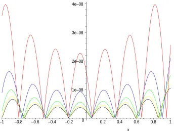
3.3 Absolute error of a Fourier-Hermite expansion using 16, 32 and 64 basis functions and 4 time steps . . . 61

3.4 Absolute error of a Fourier-Hermite call option expansion using 64 basis Functions and 4 time steps with double precision . . . 62

3.5 Absolute error of a Fourier-Hermite expansion using 32 basis functions and varying time steps with double precision . . . 64

3.6 Absolute error of a Fourier-Hermite expansion using 64 basis functions and varying time steps with double precision . . . 66

3.7 Absolute error of a Fourier-Hermite put option expansion using 64 basis Functions and 4 time steps with double precision . . . 68

4.1 An example of a normalised Fourier-Hermite expansion and the Black Scholes formula . . . 100

4.2 Absolute error of a normalised Fourier-Hermite expansion using 32 basis Functions and 4 time steps . . . 101

5.1 A graphical representation of the weight function . . . 125

5.2 A graphical view point of the interval allocation forK = 4 . . . 127

5.3 The discretization ofx_k . . . 132

5.4 The discretization ofx for K = 4 with a ﬁxed number of partitions . 137 5.5 The eﬀects of a changingη with K = 8 andN = 128 . . . 138

(13)

5.9 The eﬀects of a changingη with K = 6 andN = 128 . . . 140

5.10 The eﬀects of a changing η with K = 6 andN = 64 . . . 141

5.11 The eﬀects of a changing η with K = 6 andN = 256 . . . 141

5.12 The eﬀects of changing the Interest Rate with K = 8 andN = 128 . . 142

5.13 The eﬀects of changing the Volatility with K = 8 and N = 128 . . . . 142

5.14 The eﬀects of changing the Time to Expiry with K = 8 and N = 128 143

5.15 Approximations for Various K and N with η= 10−7 . . . 144

5.16 Adaptive Node Distribution for the ﬁrst 4 time steps when K = 8 . . 149

5.17 The discretization of x_k . . . 152

7.1 Absolute error of a Fourier-Hermite expansion using 16, 32 and 64

(14)

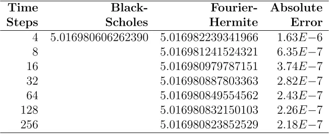
3.1 Fourier-Hermite - European call option prices for 4 time steps and

various basis functions . . . 60

3.2 Fourier-Hermite - European call option prices for 4 times and various

basis functions (with double precision) . . . 63

3.3 Fourier-Hermite - European call option prices for 32 basis functions

and various time steps . . . 65

3.4 Fourier-Hermite - European call option prices for 64 basis functions

3.5 Fourier-Hermite - European put option prices for 4 time steps and

various basis functions . . . 69

3.6 Fourier-Hermite - American put option prices for various time steps

and 40 basis functions . . . 83

3.7 Fourier-Hermite - American put option prices for 40 basis functions

and the best number of time steps . . . 83

3.8 Fourier-Hermite - American put option prices for 40 time steps and

the best basis functions . . . 84

4.1 Normalised Fourier-Hermite - European call option prices for 4 time

steps and various basis functions . . . 102

4.2 Normalised Fourier-Hermite - European call option prices for 4 time

steps and various basis functions (with double precision) . . . 103

4.3 Normalised Fourier-Hermite - European put option prices for 4 time

steps and various basis functions . . . 104

4.4 Normalised Fourier-Hermite - American put option prices for various

(15)

of time steps . . . 116

4.6 Comparison of the Fourier-Hermite expansion methods for various

American put option prices for 40 time steps and the best basis functions117

5.1 An example of the intervals of integration used for pricing an option

using 4 time steps . . . 127

5.2 European call option intervals of integration for K = 4 . . . 131

5.3 Black-Scholes - European option prices . . . 134

5.4 Interpolation method - European call option with 8 time steps and

128 partitions . . . 135

5.5 Interpolation method - European put option with 8 time steps and

5.6 Interpolation method - European call option price using ﬁxed spaced

partitions . . . 145

5.7 Comparison of ﬁxed number and ﬁxed spaced partitions for a

Euro-pean Call . . . 146

5.8 Interpolation method - European call option prices with adaptive

node distribution with an interpolating error = 10−9 . . . 148

5.9 Interpolation method - European call option prices with single

adap-tive node distribution at the ﬁrst time step with an interpolating error

= 10−9 . . . 150

5.10 Left Endpoint - European call options with 4 time steps and 32

par-titions . . . 153

5.11 Left Endpoint - European call options (for optimal η) with 4 time

steps and 32 partitions . . . 153

5.12 Left Endpoint - European call options with 4 time steps and 256

5.13 Left Endpoint - European call options (for optimal η) with 4 time

(16)

5.15 Right Endpoint - European call options (for optimal η) with 4 time

steps and 256 partitions . . . 156

5.16 Midpoint - European call options with 4 time steps and 256 partitions 158

5.17 Midpoint - European call options (for optimal η) with 4 time steps

and 256 partitions . . . 159

5.18 Trapezoidal - European call options with 4 time steps and 256 partitions160

5.19 Trapezoidal - European call options (for optimalη) with 4 time steps

5.20 Composite Simpson’s Rule - European call options with 4 time steps

5.21 Composite Simpson’s Rule - European call options (for optimal η)

with 4 time steps and 256 partitions . . . 162

6.1 Interpolation method - American put option for 100 partitions and

various time steps . . . 168

optimal time steps . . . 168

various time steps . . . 169

optimal time steps . . . 169

6.5 Interpolation method - American put option for 8 time steps and

various partitions . . . 170

6.6 Interpolation method - American put option for 8 time steps and

optimal partitions . . . 170

6.7 Interpolation method - American put option price using ﬁxed spaced

partitions for an asset price of $100 . . . 171

(17)

partitions (with an extra decimal place) for an asset price of $100 . . 173

6.11 Interpolation method - precise American put option price using ﬁxed

spaced partitions for various asset prices . . . 173

6.12 Interpolation method - American put (asset value of $100) for

adap-tive node points and 4 time steps . . . 174

6.19 Down and Out call option intervals of integration for K = 10 . . . 179

6.20 Interpolation method - Down and Out call (asset value of $100) for

ﬁxed number of partitions (N = 64) and 8 time steps . . . 180

ﬁxed number of node points (N = 128) and 8 time steps . . . 180

6.22 Interpolation method - Down and Out call for ﬁxed number of node

points (N = 256) and 8 time steps . . . 181

(18)

6.26 Interpolation method - Down and Out call for Adaptive node points

and 8 time steps . . . 185

6.27 Interpolation method - Down and Out call for Adaptive node points

6.28 Left Endpoint Quadrature - American put option for 200 partitions

6.29 Left Endpoint Quadrature - American put option for 8 time steps and

optimal partitions . . . 188

6.30 Various Quadrature Rules - American put option for 8 time steps and

6.31 Left End and Mid point Quadrature Rules - American put option

for an Asset Price of $100, 8 time steps and an optimal amount of

6.32 Left Endpoint Quadrature - Down and Out call option for 8 time steps190

6.33 Right Endpoint Quadrature - Down and Out call for 8 time steps . . 191

6.34 Midpoint Quadrature - Down and Out call for 8 time steps . . . 192

6.35 Trapezoidal Quadrature - Down and Out call for 8 time steps . . . . 193

6.36 Composite Simpson’s Quadrature - Down and Out call for 8 time steps194

6.37 Comparing Quadrature - Down and Out call (asset value of $100) for

8 time steps and 256 partitions . . . 195

C.1 European call option (Interpolation Polynomials) with K = 8, N =

64 and asset value of $80 . . . 244

(19)

128 and Asset value of $80 . . . 252

(20)

C.26 European call option (Interpolation Polynomials) with K = 16,N =

C.31 European call option price using ﬁxed spaced nodes with K = 8 . . . 260

C.32 European call option prices with adaptive node distribution with an

interpolating error= 10−6 . . . 261

(21)

C.38 European call option prices with single adaptive node distribution at

the ﬁrst time step with an interpolating error= 10−6 . . . 264

C.45 Interpolation method - Down and Out call (asset value of $100) for

C.47 Interpolation method - Down and Out call for ﬁxed number of node

points (N = 256) and 8 time steps . . . 271

C.50 Interpolation method - Down and Out call (asset price of $100) for

(22)

C.52 Interpolation method - Down and Out call for Adaptive node points

(23)

Introduction

The pricing of derivative securities, such as options, has in the past three decades,

encroached into the world of science. Many mathematicians, physicists and

statisti-cians have contributed their methodologies and techniques to the world of ﬁnance.

These methods, usually used in engineering and the physical sciences, have been

aptly adapted to problems in the ﬁnancial world.

The major issue confronting investors is security of their assets or ﬁnancial position.

A wheat grower may want to sell his/her crop in the future at a predetermined

price and not wait until the crop is ready to sell (at a price below expectation). An

investor would like to buy or sell shares in a company ABC for a predetermined

price in the future.

Given these issues, pricing of derivative securities is not so simple. With diﬀerent

underlying assets to protect, the condition of ﬁnancial markets changing from

na-tion to nana-tion, investor sentiments diﬀering due to human feelings and other factors

inﬂuencing security prices, mathematical modeling can be complex.

In creating a ﬁnancial instrument involving the risk of an underlying asset, the

following aspects must be taken into consideration when modeling;

i. An understanding of the underlying asset,

(24)

iii. Other conditions involved in the markets where the ﬁnancial instrument and

the underlying asset are traded. Examples of such conditions include trading

periods, transaction costs and interest rates.

Later in this chapter, an investigation is made into various methods and techniques

used to assist in the pricing of derivative securities. In an eﬀort to combat the

com-plexities of models designed, many authors place conditions and constraints such

that solutions/approximations can be made.

The thesis will concentrate on the area of pricing using a path integral framework.

The use of path integrals has been commonplace in science for many years since

the creation of the path integral in Feynman (1942). Its application to ﬁnance, in

particular the pricing of derivative securities, has been less common. The thesis will

oﬀer various alternative techniques to solve a particular path integral model. One of

the major advantages of the methods presented is the high accuracy achieved, very

eﬃciently and with relatively low computational eﬀort.

The remainder of this introduction includes a section 1.1 of commonly used terms.

Section 1.2 gives a brief summary of the basic concepts used in the pricing of options.

An explanation of factors which aﬀect Options and their pricing are also given.

Sec-tion 1.2 also gives a thorough review of the literature for non path integral modeling

of option pricing.

Section 1.3 reviews option price modeling with an emphasis on Path Integrals. It is

hoped that the review in section 1.2 and 1.3 will allow the reader to appreciate the

vastness of the topic at hand. We ﬁnally state the objectives and aims of this thesis

(25)

1.1 Common Terminology

The following section gives a very brief overview of the basic terms and concepts

involved in option pricing. If further understanding of the basic areas of ﬁnancial

derivatives and the markets they trade in is required, then Hull (2006) and Wilmott

(1999) are excellent resources. Most of the terms and concepts within this section

are sourced from Atkinson (1989), Kreyszig (2006), Hull (2006) and Wilmott (1999).

The following is a list of commonly used terms within this thesis.

Commodities: Commodities are usually raw products such as precious metals, oil,

food products etc.

Forward Contract: A forward contract is an agreement where one party promises

to buy an asset from another party at some speciﬁed time in the future and at some

speciﬁed price.

Futures Contract: A futures contract is similar to a forward contract with the

only diﬀerence being that they are traded on an exchange and are marked to market.

Options: Gives one party the opportunity to buy or sell an asset from/to another

party at a prearranged price.

Call Options: The holder has the right to buy an asset by a certain date for a

certain pre-agreed price.

Put Options: The holder has the right to sell an asset by a certain date for a

certain pre-agreed price.

European Options: Options that can only be exercised at the expiration date.

American Options: Options that can be exercised at any time up to the

expira-tion date.

Barrier Options: Options of an exotic type, in which the payoﬀ depends upon

the reaching or crossing of a barrier (predetermined price) by the underlying. These

options include call options and put options, and are similar to common options in

many respects. Barrier options become active/inactive when the underlying crosses

(26)

Underlying: The ﬁnancial instrument on which the derivative value depends. The

option payoﬀ is deﬁned as some function of the underlying asset at expiry.

Strike or Exercise Price: The amount at which the underlying can be bought

(call) or sold (put).

Expiration or Expiry Date: Date on which the derivative can be exercised or

date on which the option ceases to exist or give the holder any rights to act.

Intrinsic Value: The payoﬀ that would be received if the underlying is at its

cur-rent level when the derivative expires.

In the Money: An option with positive intrinsic value.

Out of the Money: An option with no intrinsic value, only time value.

At the Money: A call or put with a strike that is close to the current asset value.

Hedging: A strategy to Establish a guaranteed future price of a commodity.

Speculating: Investors wishing to take a position in the market. Either they are

betting that the price will go up or they are betting that it will go down.

Arbitrage: Involves locking in a riskless proﬁt by simultaneously entering into

transactions in two or more markets.

Volatility: Is the term given to represent the standard deviation of the

instanta-neous return of the underlying.

Fourier Analysis and Series: Fourier Analysis concerns the study of periodic

phenomena. Fourier Series is a series which represents complicated functions in

terms of simple periodic functions.

Mathematical Interpolation: Mathematical interpolation is the selection of a

function p(x) from a given class of functions satisfying some smoothness conditions

in such a way that the graph of y =p(x) passes through a ﬁnite set of given data

points.

Quadrature: The quadrature of a geometric ﬁgure is the determination of its area.

(27)

1.2 Options and Option Pricing

To appreciate the content of the following thesis, an introduction to some of the

basic concepts is worthwhile. The concepts covered in this section include aspects

of option pricing and the mathematics presented throughout the thesis. To a

math-ematician some of the methods used in the thesis are quite novel. But to understand

the problem at hand, an introduction to terms and concepts used in option pricing

may be required.

The term Risk Management is sometimes used to describe the security of

invest-ments. As people insure their valuable possessions such as houses, cars and boats,

investors need to secure their assets and/or ﬁnancial position by using ﬁnancial

in-struments such as options (contingent claims).

Within the ﬁnancial world, there are various assets, and many variants that aﬀect

the value of an asset. Some examples of assets that can be secured and the factors

that aﬀect the value of them, include:

• Shares

• Commodities such as Wheat, Wool, Sheep, Electricity, etc

• Bonds

• Stock Exchange Indices

• Foreign Exchange

• Interest Rates

• Volatility.

Given the nature of assets and the variants, the pricing of ﬁnancial instruments

such as options is sometimes complex and time consuming. Adams, Booth, Bowie

& Freeth (2003) states various factors that aﬀect the pricing of options. The factors

(28)

• Exercise Price

• Underlying Asset Price

• Time to Expiry

• Volatility

• Interest Rates

• Incomes & Dividends.

Adams et al. (2003) brieﬂy explains the meaning of each factor but also describes

how each factor aﬀects the value of the option (Put and Call). In later chapters, we

explain and analyse the eﬀects of these factors on the price of options.

Options are common ﬁnancial instruments which allow one party to buy/sell assets

from another party for a particular price. As described, many factors inﬂuence the

value of the option. The remainder of this section will take a detailed look at the

modeling of options as well as the techniques used to determine the value of an

option.

Since the development of the pricing of derivative securities by Black & Scholes

(1973) and Merton (1973), the literature has become vast. This area of ﬁnance has

developed to the point where science has taken a grasp and inﬂuenced the creation

of various models and the techniques to solve them. With the Black, Scholes and

Merton developments of their formula to the development of models which

incorpo-rate Jump Diﬀusion parameters, science and especially mathematics, have been at

the forefront of pricing ﬁnancial instruments (options).

The literature provides a variety of techniques to solve various option prices. Some

of the major methods used include (in no particular order):

1. Lattice Structures (Trees)

(29)

3. Quadrature

4. Solutions to partial diﬀerential equations (PDE’s)

5. Martingales and other probabilistic methods.

With the development of the Black and Scholes partial diﬀerential equation (PDE)

and the analytic solution (formula), the mathematical/scientiﬁc world became

in-volved. The further development and extensions of the Black-Scholes PDE and

the creation of other types of options (that is, exotic, barrier and path dependent

options) has led to other mathematical methods for their modeling and analysis.

Chapter 2 gives a detailed presentation of the Black and Scholes paradigm and the

development of the PDE leading to the Black and Scholes formula.

Since Black & Scholes (1973) and Merton (1973), the literature for pricing derivative

securities has ﬂourished. The techniques and methodologies employed are

numer-ous and varied. The most common techniques used include simulation, particularly

Monte Carlo and discretization methods like binomial and trinomial trees, and ﬁnite

diﬀerences. The varying techniques employed are dependent on the equations to be

solved. The most common form of equations used are diﬀerential equations.

How-ever, in recent times, the use of path integrals has increased and various techniques

to solve these integrals have been developed.

Other techniques are also employed due to the creation of other types of securities.

These securities are sometimes complex compared to the original warrants described

by Black, Scholes and Merton. However, some of these securities are based on the

Black and Scholes paradigm. They are based on similar assumptions and conditions

as described in Chapter 2.

This section will present the inﬂuential and relevant works in the option pricing

world. Some of the methods and techniques developed over the years have shown

the multitude of mathematical adaptations used to procure an option price. This

(30)

ad-vancement of option pricing.

The ground breaking and deﬁning work by Black, Scholes and Merton, paved the

way for many changes in the management and modeling of risk. Many subsequent

authors have gone on to extend and modify the early work of Black, Scholes and

Merton. Along with these new works, has been the creation of new ﬁnancial

instru-ments (and options) based on the models and theories of these authors.

Another inﬂuential paper is that of Cox, Ingersoll & Ross (1985) who present a

theory of the term structure of interest rates. This paper is of great importance to

the ﬁnancial world, as it has led to other types of modeling in ﬁnance, not just those

related to Black, Scholes and Merton’s work. They explain the term structure of

interest rate as a relationship among the yields on default-free securities, that diﬀer

only in their term to maturity. By oﬀering a complete schedule of predicted interest

rates across time, the term structure embodies the markets’ anticipations of future

events.

The authors present a description of the previous works on the term structure of

interest rates. Cox, Ingersoll and Ross incorporate general equilibrium theory, in

combination with the previous studies to develop their term structure of interest

rates. It is worth mentioning the work of Maghsoodi (1996) who extends the Cox,

Ingersoll and Ross model to incorporate time-varying parameters. The work by

Cox, Ingersoll and Ross and related authors shows that not all risk management

and ﬁnancial instrument modeling revolves around early methods and techniques

of Black, Scholes and Merton, and that there are other methods and techniques to

investigate and that model ﬁnancial risk.

The rest of this section will describe the modeling of other authors who have based

their works mainly around that of Black and Scholes, and Merton. Most of the

modeling is based on extensions and alternatives of their basic models. Other

(31)

are some models with solutions to ﬁnancial instruments using numerical methods,

especially for American options. In reviewing these extended and modiﬁed models,

the various types of methods and techniques used are clear. The authors presented

various diﬀerences to the earlier models. Popular methods included the relaxation of

assumptions, the introduction of real market occurrences and various diﬀering

meth-ods and techniques to solve the old models. The following paragraphs are grouped

in such a way that these variations are made clear.

An appropriate extension/modiﬁcation to the work of Black & Scholes (1973) was

devised by Hyland, McKee & Waddell (1999) to incorporate time-dependent interest

rates and volatility. The authors present some interest rate and volatility models to

illustrate their work. These models are very general time-dependent equations and

are not indicative of the typical interest rate and volatility structures.

Silverman (1999) and Garven (1986) present alternative methods to ﬁnd a solution

to the Black and Scholes PDE, namely

∂V ∂t +

1 2σ

2_S2∂2V

∂S2 +rS ∂V

∂S −rV = 0. (1.1)

where V is the option price, t is time, σ is the volatility associated with the asset

which has a value S and r is the interest rate.

Silverman’s involves the use of Green’s function and Garven’s presentation is in

view of the risk neutrality arguments presented by both Cox & Ross (1976) and

Ru-binstein (1976). It is clear that there are alternative methods to solve (1.1) other

than the conversion to the heat transfer equation method used by Black and Scholes.

In the following paragraphs, a summary of various types of European option models

will be made. These descriptions will show the types of modiﬁcations and extensions

to option pricing models that have been performed over the years, with particular

reference to the Black-Scholes equation. These models present changes to the Black

(32)

of modeling options for real market scenarios. As stated previously, the advantage of

the Black, Scholes and Merton model is that the option price is easily found. Even

though these models are more realistic, they do require extensive computational

effort. In some cases, exact solutions are difficult to find.

Jennergren & Naslund (1996) and Merton (1976) present an extended Black-Scholes

model to incorporate a class of option with stochastic lives (options which may

be canceled but the underlying stock retain their value). This is an appropriate

modiﬁcation, as options may cease to exist due to company mergers, bankruptcy,

and employee resignations (for an employee class option) as examples. The

intro-duction of arbitrage is a useful modiﬁcation to the modeling of ﬁnancial risk. Ilinski

(1999) allows the possibility of virtual arbitrage in his modiﬁed Black-Scholes model.

However, by allowing arbitrage possibilities, one would have to be realistic and have

to consider the cost(s) involved in obtaining such a riskless position. So, another

popular method of extending the Black-Scholes equation (or any other ﬁnancial

in-strument model) is the introduction of transaction costs or fees. There have been

various modiﬁed models presented over the years to incorporate the eﬀects of

trans-action costs. One of the ﬁrst and most popular works in regards to transtrans-action costs

was that of Hodges & Neuberger (1989). Later, Davis, Panas & Zariphopoulou

(1993) developed a model for European options with transaction costs, with Davis

& Zariphopoulou (1995) presenting a similar model for American options. Whalley

& Wilmott (1997) produced an eﬃcient and simpler hedging strategy to be

calcu-lated. One of the main problems in analysing these types of models is, that they may

be too complex and the question as to whether there is a method to ﬁnd a simpler

solution. Chao, Jing-Yang & Sheng-Hong (2007) use a Markov chain approximation

to compute Barrier option prices with transaction costs. Given new methodologies

and techniques, instead of ﬁnding a precise solution for a complex model,

deter-mining an imprecise result, together with an estimate of the imprecision, will allow

(33)

Another assumption that can be modiﬁed/manipulated is the structure of volatility.

The original Black and Scholes model used a constant volatility for the stock price,

which was used for the purpose of simpliﬁcation. However, stock/asset volatilities

have complex structures and it would be appropriate to represent these complex

volatility structures (i.e. stochastic volatility) in the option pricing models. One of

the most popular models developed was by Heston (1993). The Heston Model is

used by many authors when comparing their own models and techniques involving

stochastic volatility. Heston shows there is a bias between volatility and the spot

asset price. Therefore, he incorporates this into his model. Finally, analytical forms

are found for the various PDE’s using characteristic functions which are easy to

compute.

Some other models presented to incorporate varying volatility structures worth

men-tioning include Chalupa (1997), Sircar & Papanicolaou (1998), Kurpiel & Roncalli

(1998) and Zuhlsdorﬀ (2001). In recent times, Medvedev & Scaillet (2007) derive

implied volatilities for options under a two-factor jump-diﬀusion stochastic

volatil-ity. Hilber, Matache & Schwab (2005) oﬀer a unique approach to solving option

prices under stochastic volatility. They oﬀer an algorithm based on a sparse wavelet

space discretization.

Given the extensive works by the previous authors in modifying or extending the

work of Black and Scholes, and Merton, there have been presentations of other

ﬁ-nancial instrument models (and in particular, other option pricing models). One of

these is the modeling of Exotic options. These options are non-standard options,

and have been examined extensively. This thesis will examine exotic (American and

Barrier types) along with the Vanilla (European type) options.

There have been numerous exotic option pricing models presented including that

of Carr, Ellis & Gupta (1998) who develop static hedges for several exotic options

using standard options. In this area, the work of Neuberger & Hodges (2000) in

(34)

approach for rational bounds on the pricing of exotic options is worthy of

exam-ination. Penaud, Wilmott & Ahn (1998) extend a Vanilla Passport option to add

various exotic features to that option. The authors present seven diﬀerent types of

exotic passport options, using the same assumptions as used in deriving the

Black-Scholes equation. Schoutens & Symens (2003) present a Monte Carlo simulation

method to price exotic options with stochastic volatility.

An interesting exotic option pricing model is proposed by Geman (2001). The

au-thor develops a technique to ﬁnd the price of a type of exotic option called an Asian

option (there is also the development of a Barrier option). The technique oﬀered

involves the use of Laplace transforms and of a time-changed squared Bessel

pro-cess. Geman presents some numerical work, comparing the author’s results to an

equivalent Monte Carlo simulation.

Finally, some of the more recent techniques used in approximating ﬁnancial

instru-ment pricing models is via the use of Martingale methods and game theory. Musiela

& Rutkowski (1997) present numerous ﬁnancial instrument models via the use of

Martingale Methods. Prigent, Renault & Scaillet (2004) also address the problem of

option pricing (with discrete re-balancing) using Martingale measures. Henderson

(2005) presents some Martingale measures to incomplete stochastic volatility

mod-els. The use of Martingale methods and game theory reiterates that the modeling of

ﬁnancial instrument (option) pricing is open to various methods and techniques.

Ols-der (2000) develops a technique for the pricing of options using game theory. The

author oﬀers one model for a two player system, with the players being nature and

the investor. The second model consists of three players, being nature, the investor

and the bank (whose presence forces the introduction of transaction costs).

So far the review has presented models for corporate liabilities, European options

and exotic options. One of the most common ﬁnancial instruments (and option)

is the American option. These options allow the owner to buy or sell the

(35)

literature in the mathematical modeling of American options, with the main issue

concerning when to exercise an option. This problem is known as the early exercise

option.

One of the ﬁrst American option pricing models to be presented is that of Brennan

& Schwartz (1977). Their work has also been extended and modiﬁed over the years.

Another two relevant American option pricing models presented are by Geske &

Johnson (1984) and Kim (1990). The following paragraphs will summarise their

work.

Brennan & Schwartz (1977) conﬁrms that the American put option obeys the

Black-Scholes equation. The authors then describe and state a numerical method to solve

the Black-Scholes equation for an American option. The solution for the American

option diﬀers greatly to the European option, as an American option can be

exer-cised at any time up to the exercise date. Brennan and Schwartz apply their model

against some historical data. They compare the put result against the equivalent

Black-Scholes European put option. This comparison seems to be irrelevant, as a

European option can only be exercised on the exercise date. Cox, Ross & Rubinstein

(1979) oﬀers a Binomial tree approach to various options, including an American

put. They argue that their alternative approach to Brennan & Schwartz (1977) is

simpler and in most cases computationally more eﬃcient.

Geske & Johnson (1984) developed an analytical approximation for an American

put option. They argue that numerical solutions are expensive, which may have

been the case in the 70’s and 80’s. The analytical solution presented by Geske and

Johnson is

P =Xw₂−Sw₁ (1.2)

where w₁ and w₂ may be represented as a Taylor series, X is the exercise price and

(36)

In devising this solution, Geske and Johnson determine at each instant, dt, the put

will be exercised if, the put has not already been exercised and the payoﬀ from

exer-cising the put equals or exceeds the value of the put if it is not exercised. The authors

go on to present formula evaluations and applications, comparing their results to

those of Parkinson (1977) and Cox & Rubinstein (1984). In comparing their results,

the authors state that the option values yielded are within one penny of each other.

They also note that the European value is close to the American value, where the

American option would be more valuable when the early exercise option is taken.

They also indicate that the analytical solution they oﬀer is faster to compute by a

factor of 10 compared to the standard numerical methods. At the time of the model

presentation, the analytical approximation may have been faster. Analytical

approx-imations has its advantages as prices can be evaluated precisely and can be used to

compare against other methods and techniques. But with high-speed computers and

eﬃcient numerical methods, the argument of analytical approximations being faster

to calculate is now out-dated, however analytic solutions do provide valuable insight.

Kim (1990) oﬀers a diﬀering analytical evaluation of an American put via the use

of numerical methods. Kim questions the Geske & Johnson (1984) solution, as Kim

states it is yet to be shown that an analytical solution to an American put value can

be obtained as the sum of an inﬁnite series of functions.

The integral equation presented in Kim (1990) cannot be solved explicitly, however,

it can be solved numerically. In determining the optimal exercise boundary, B(s),

the computation of the American put value is achieved by straight forward

numeri-cal integrations. Some of the techniques oﬀered in this thesis may be applied to the

integral equation presented in Kim (1990).

There has also been modeling of American options using various other methods and

techniques. Jaillet, Lamberton & Lapeyre (1990) verify the modeling of Brennan

& Schwartz (1977) with the use of variational inequalities. El Karoui & Karatzas

(37)

of their work is an extension of Bensoussan (1984). As discussed previously in this

review, Davis & Zariphopoulou (1995) present a model for American options with

transaction fees. Coleman, Li & Verma (1999) oﬀer a Newton method for

Ameri-can option pricing. Their work is based around improving the work of Brennan &

Schwartz (1977). These models show that there are various mathematical methods

and techniques that can be applied to the pricing of American options.

Other models and solutions using numerical methods worth noting are Siddiqi,

Man-chanda & Koˇcvara (2000), who deﬁne an application of an eﬃcient algorithm for a

numerical solution for American options. The solution, like that of many authors

previously, is based on the Black-Scholes equation. Stamicar, ˇSevˇcoviˇc & Chadam

(1999) ﬁnd a numerical approximation for an early exercise boundary for an

Ameri-can put option near expiry. Zhao, Davison & Corless (2007) design a compact ﬁnite

diﬀerence method for pricing American options. The authors oﬀer three types of

ﬁnite diﬀerence methods and the results compare favourably to the existing

Crank-Nicolson methods.

Sullivan (2000) uses Gaussian quadrature to evaluate the price of an American put

option. Initially the author presents approximations for a European put option

using a Binomial Tree, Trapezoidal, Simpson’s and Gauss-Legendre methods, with

the Simpson and Gauss-Legendre methods working quite well. The Gauss-Legendre

quadrature is then applied to the American put option using Chebyshev

approxi-mations. Thorough analysis of convergence, accuracy and speed are presented and

comparisons to analytical methods are made. Some of the quadrature described

in Sullivan (2000) will be applied to a path integral representation of various types

of options in the thesis (Chapter 5 and 6).

In describing these models in the last couple of paragraphs, it is clear that the

mod-eling of American options is more complex than the modmod-eling of European options

since American options can be exercised at any time up to the expiry date.

(38)

be exercised) is just as important as the value of the option itself.

In collating this review of pricing of ﬁnancial instruments like options, it is clear that

ﬁnancial instruments are becoming complex to model and to price. This review was

presented to give an overview of the changing landscape of option pricing. An area

that has not been presented thus far is the use of Path Integrals which is the main

emphasis of the thesis.

Path Integrals have been used in the area of science for many years. In the world

of option pricing it has only been in the last decade or so that the path integral has

been used to model the price of an option. The following section will give a review

of the literature presented so far. It is envisaged that the reader has some basic

knowledge and understanding of path integrals.

1.3 Option Pricing and Path Integrals

The use of path integrals has developed into a viable option pricing model

represen-tation in the past decade or so. Since the creation of the Black-Scholes PDE and the

various techniques to solve (1.1), authors have attempted to model vanilla and non

vanilla options in alternative forms. Path integrals has been one of the alternative

methods.

Path integrals have been used in various areas of science over the years, especially

in quantum physics. One of the advantages of using path integrals is the variety of

techniques used to solve them. From Monte Carlo simulation to various quadrature

methods, the techniques have been developed and applied to ﬁnance.

The following review will present the use of path integrals to model and the

tech-niques to evaluate option prices. One of the early uses of a path integral in derivative

security pricing was from Makivic (1994). The author presents a Monte Carlo

(39)

Makivic also states that the main advantages of a path integral approach are:

(1) partial derivatives of the price with respect to all of the input parameters can

be computed in a single simulation,

(2) results for multiple setsof parameters can be computed in a single simulation,

and

(3) suitability for implementation on a parallel or distributed computing

environ-ment.

It must be said that his assertions are correct for a path integral approach using

Monte Carlo simulation to evaluate the price. The best results show errors of order

10−4.

Baaquie (1997) presents a path integral approach to option pricing with stochastic

volatility. Baaquie generalises the results of Hull & White (1987) for cases when

the stock price and volatility have non-zero correlation. Ingber (2000) also presents

a path integral approach to options with stochastic volatilities. The author uses an

Adaptive Simulated Annealing approach to determine the behaviour of diﬀusion.

This behaviour is determined by daily Eurodollar future prices and implied

volatil-ities. An algorithm called PATHINT is used to evaluate prices.

Linetsky (1998) oﬀers a path integral approach to ﬁnancial modeling and option

pricing. The author states that ”the path integral formalism constitutes a

conve-nient and intuitive language for stochastic modeling in ﬁnance”. Linetsky presents

various path integrals, including a framework for the Black-Scholes paradigm path

dependent options and multi-asset derivatives. The author ﬁnally develops

evalu-ations for various options using analytical approximevalu-ations and numerical methods

(Monte Carlo simulation and/or discretization schemes).

Some authors have investigated the use of path integrals to model path dependent

(40)

options (Asian options and occupation time derivatives). The method of partial

averaging reduces the dimension of the integral. The evaluation can be performed

by Monte Carlo simulation methods. Baaquie, Corian`o & Srikant (2003) also oﬀer a

path integral approach to solve for path dependent options. They build their model

using the Black-Scholes paradigm and then extend it to create more complex

secu-rities such as exotic and path dependent options. Baaquie et al. (2003) evaluate the

option prices by Monte-Carlo simulation. Bormetti, Montagna, Moreni & Nicrosini

(2006) also present a path integral framework to evaluate (via Monte Carlo

simula-tion) prices for various path dependent options.

An interesting application using a path integral approach is oﬀered by Otto (1999).

The author presents a model to price interest rate derivatives. Path integrals for the

short term and bond option are developed. Otto suggests two techniques to solve

these derivatives, they are a lattice method or the use of Monte Carlo simulation.

Bennati, Rosa-Clot & Taddei (1999) develop a path integral approach for various

stochastic equations that best represent ﬁnancial markets. The path integrals are

designed to cater for one and multi dimensional cases. The authors then present

some analytic results for various models such as Black-Scholes, Cox-Ingersoll-Ross

and others. Rosa-Clot & Taddei (2002) oﬀer numerical methods to price some of

the derivative securities presented in Bennati et al. (1999). Rosa-Clot and

Tad-dei use two methods to evaluate prices, Monte Carlo simulation and deterministic

evaluations (quadrature rules). The deterministic evaluations has its advantages

in low dimensional problems but in high dimensions the technique has issues with

large matrix dimensions. Various options (European options , Zero-coupon bonds,

Caplets, American options and Bermudan swaptions) are priced.

Some authors have investigated the use and evaluation of path integrals to price

op-tions using unique and less common techniques. Kleinert (2002) presents a Natural

Martingale for non-Gaussian ﬂuctuations of the underlying. Decamps, De Schepper

(41)

manage-ment. Chiarella, El-Hassan & Kucera (1999) present an evaluation of a European

and American option in a path integral framework. The novel approach to the

eval-uation is the use of a Fourier-Hermite series. The technique takes into consideration

the form of the integrand of the path integral (1.3),

fk−1(ξ_k₋₁) = e

−rΔt

√

π

_∞

−∞

e−(ξk−μ(ξk−1))2_fk₍√_{2Δt ξ}

k)dξk. (1.3)

The Gaussian in the integrand is in the form of the weight of a Hermite orthogonal

polynomial. The price function, fk_(ξ

k), is expanded into a Fourier-Hermite series. This series is continuous and is a diﬀerentiable representation of the underlying.

Given the form of the Fourier-Hermite series, the Deltas are easily found as well as

the option price.

In Chapter 2 we present the development of the path integral (1.3). Chapter 3, in

this thesis, gives a thorough overview of the technique used to ﬁnd the option price.

In this overview of the technique, errors were found in the formulation and in the

results presented. The path integral is formed using an application of Ito’s Lemma.

Chapter 4 oﬀers a modiﬁcation to the technique used to evaluate the option price.

The alternative method uses normalised Hermite orthogonal polynomials. The use

of the normalised polynomials has its advantages, especially when a large number

of basis functions are used.

An extension of the previous approach is oﬀered by Chiarella, El-Hassan & Kucera

(2004) to incorporate the evaluation of point barrier option prices. The path integral

is very similar with the only diﬀerence being the integral domain. The path integral

(1.3) with a ﬁnite domain, namely,

fk−1(ξ_k₋₁) = e

−rΔt

√

π

_z_k,u

zk,l

e−(ξk−μ(ξk−1))2_fk₍√_{2Δt ξ}

k)dξk, (1.4)

(42)

z_k,l = ln (bk,l)

σ_k2Δt_k, and zk,u =

ln (b_k,u)

σ_k2Δt_k, (1.5) fork =K−1, . . . ,1 withb_k,l andb_k,ubeing the lower and upper barriers respectively, at time step k.

Chapters 5 and 6 oﬀer alternative techniques to evaluate the same path integral

framework (1.3) and (1.4). Prices are approximated for European, American and

Barrier options. The techniques take into account the form of the integrand such

that interpolation polynomials and various quadrature rules can be used. The

tech-niques employed are highly accurate and very fast to compute.

Given the literature review presented in this thesis, it is clear that the methods

and techniques used in evaluating the option price are vast. From the early days of

Black, Scholes and Merton to the introduction of many scientiﬁc approaches, option

pricing is a growing area in both ﬁnance and mathematics. Path integrals in ﬁnance

is relatively new in comparison, with the last decade seeing an increase in activity.

Path integrals have been used in areas such as quantum physics for many years since

(43)

1.4 Thesis Objectives

The thesis is based around the path integral framework oﬀered by Chiarella et al.

(1999). In their method, the underlying is expanded into a Fourier-Hermite series.

At each time step, the coeﬃcients of the series are determined in a backward

recur-sive manner, using recurrence relations. These relationships are formed utilising the

orthogonal properties of Hermite orthogonal polynomials. In Chapter 3, an

anal-ysis of the method described by Chiarella et al. is presented. This will assist in

understanding the remaining chapters and comparison of techniques used to solve

the same problem.

The first approach is similar to that offered by Chiarella et al. The main difference

being the use of normalised Hermite orthogonal polynomials. A set of recurrence

relations are formed, as with the previous method. The beneﬁts of using the

nor-malised polynomials are the form of the recurrence relations as well as the speed to

ﬁnd accurate results (especially for the European option). Some relations have one

less exponential term. Given this fact, the speed of computation should be improved

for a large number of basis functions.

The next approach, using the same path integral framework, also converts the

un-derlying price at each time step. The price is represented by a series of interpolation

polynomials. In this method, integration is performed only once, at the beginning

of the process. Using the result of the integration and the interpolation polynomial

coeﬃcients found, the option price is evaluated. This process is repeated at each

time step. The method requires no transformations and is quite straight forward to

implement. The path integral framework is converted from an inﬁnite interval to a

ﬁnite interval.

The major issues arising from this method include, the determination of the interval

of integration and the node point allocation. The problem of the interval of

(44)

distribution will vary depending on the derivative security being priced. Similar to

Chiarella et al., the resultant derivative security price is continuous and inﬁnitely

diﬀerentiable allowing for fast and accurate evaluation of the hedge ratios (if

re-quired). The major advantage of this method is the very high accuracy obtained

and the easy adaptation for American and Barrier type options.

The ﬁnal approach uses traditional quadrature rules such as the trapezoid and

Simp-son’s rule. Using a similar set up to that of the previous technique, a quadrature

scheme is formed to represent the derivative security price at each time step. The

rules used show that accurate results can be found in relatively quick time. Issues as

those that have arisen in the previous approach such as node allocation also exists

in this approach. The quadrature rules can also be easily applied to American and

Barrier type options.

The thesis is a numerical investigation of the path integral framework. The thesis will

emphasise the performance and accuracy of each of the methods for the framework

and particular parameters. Trade oﬀs between accuracy and computational eﬀort

are addressed. The ease of implementation (in the case of the European options)

allows an insight into the behaviour and performance of the method for the path

integral framework and more complex options like, American put and down and out

(45)

The Black and Scholes Paradigm

This chapter shows the evolution of the Black & Scholes (1973) paradigm. It begins

with the major assumptions in which a derivative security like an option is modeled

and priced. We present the formulation of the Black and Scholes equation (a partial

diﬀerential equation) using a replicating portfolio. In deriving the Black and Scholes

equation, a formula is presented for both a European Call and a Put option. Finally,

the development of the Chiarella et al. (1999) path integral is presented, which is