Block Ciphers and Automatic Enumeration of (Related-key)
Differential and Linear Characteristics with Predefined Properties
Siwei Sun1,2, Lei Hu1,2, Meiqin Wang3, Peng Wang1,2, Kexin Qiao1,2, Xiaoshuang Ma1,2, Danping Shi1,2, Ling Song1,2, Kai Fu3
1
State Key Laboratory of Information Security, Institute of Information Engineering, Chinese Academy of Sciences, Beijing 100093, China
2
Data Assurance and Communication Security Research Center, Chinese Academy of Sciences, Beijing 100093, China
3Key Laboratory of Cryptologic Technology and Information Security,
Ministry of Education, Shandong University, Jinan 250100, China {sunsiwei,hulei}@iie.ac.cn,[email protected],
{wpeng,qiaokexin,maxiaoshuang,shidanping,songling}@iie.ac.cn
Abstract. In this paper, we investigate the Mixed-integer Linear Programming (MILP) modelling of the differential and linear behavior of a wide range of block ciphers. We point out that the differential behavior of an arbitrary S-box can be exactly described by a small system of linear inequalities.
Based on this observation and MILP technique, we propose an automatic method for finding high probability (related-key) differential or linear characteristics of block ciphers. Compared with Sunet al.’s heuristicmethod presented in Asiacrypt 2014, the new method is exactfor most ciphers in the sense that every feasible 0-1 solution of the MILP model generated by the new method corresponds to a valid characteristic, and therefore there is no need to repeatedly add valid cutting-off inequalities into the MILP model as is done in Sunet al.’s method; the new method is more powerful which allows us to get theexact lower boundsof the number of differentially or linearly active S-boxes; and the new method is more efficient which allows to obtain characteristic with higher probability or covering more rounds of a cipher (sometimes with less computational effort).
Further, by encoding the probability information of the differentials of an S-boxes into its differential patterns, we present a novel MILP modelling technique which can be used to search for the character-istics with the maximal probability, rather than the charactercharacter-istics with the smallest number of active S-boxes. With this technique, we are able to get tighter security bounds and find better characteristics. Moreover, by employing a type of specially constructed linear inequalities which can removeexactly onefeasible 0-1 solution from the feasible region of an MILP problem, we propose a method for automatic enumeration ofall (related-key) differential or linear characteristics with some predefined properties,
e.g., characteristics with given input or/and output difference/mask, or with a limited number of active S-boxes. Such a method is very useful in the automatic (related-key) differential analysis, truncated (related-key) differential analysis, linear hull analysis, and the automatic construction of (related-key) boomerang/rectangle distinguishers.
The methods presented in this paper are very simple and straightforward, based on which we implement a Python framework for automatic cryptanalysis, and extensive experiments are performed using this framework. To demonstrate the usefulness of these methods, we apply them to SIMON, PRESENT, Serpent, LBlock, DESL, and we obtain some improved cryptanalytic results.
Keywords: Automatic cryptanalysis, Related-key differential cryptanalysis, Linear cryptanalysis, Mixed-integer Linear Programming, Convex hull, Enumeration
1
Introduction
evaluation with respect to the differential and linear attacks has become a basic requirement for a newly designed block cipher to be accepted by the cryptographic community.
Matsui’s branch and bound search algorithm [23] is one of the most powerful and classic methods for obtaining a security bound with respect to differential and linear attack. However, in some cases this method is impractical. Calculating the minimum number of active S-boxes is another way to evaluate the resistance of a block cipher against the differential and linear attack [24–29]. Searching for differential and linear char-acteristics is not only performed in basic differential and linear attacks, but also is indispensable in some new cryptanalytic techniques such as the rebound attack [30] and the sieve-in-the-middle technique [31]. Moreover, some new technique for cryptanalysis (e.g., the biclique attack [32]) and some symmetric-key cryptographic schemes which can be designed based on block ciphers (e.g., the authenticated encryption schemes) make the related-key model more important and highly relevant to the design and cryptanalysis of symmetric-key primitives. Therefore, methods which can be used to evaluate the security of a block cipher with respect to the (related-key) differential and linear attacks, and search for (related-key) differential or linear characteristics are of great importance. In fact, this direction of research has got much attention from many cryptanalysts [23, 33–38].
Mouhaet al.[39] and Wuet al.[40] translated the problem of counting the minimum number of differential-ly active S-boxes, into an MILP problem which can be solved automaticaldifferential-ly with open source or commercialdifferential-ly available MILP solvers. This method has been applied in evaluating the security against (related-key) dif-ferential attacks of many word-oriented symmetric schemes, as well as in searching for linear or difdif-ferential characteristics with specific patterns [41, 42]. By introducing bit-level representations, Winnenet al.[43] and Sunet al.[44] extended Mouhaet al.’s framework, and presented methods for counting the minimum number of differentially active S-boxes of bit-oriented block ciphers both in the single-key and related-key models. We notice that such MILP based methods are also mentioned or used in the recent analysis and design of several authenticated encryption schemes [25, 42, 45–50].
In Asiacrypt 2014, two systematic methods for generating linear inequalities describing the differential properties of an arbitrary S-box were given in [51]. With these inequalities, the authors of [51] were able to construct an MILP model whose feasible region is a more accurate description of the differential behavior of a given cipher. Based on such MILP models, the authors of [51] proposed a heuristic algorithm for finding (related-key) differential characteristics, which is applicable to a wide range of block ciphers. However, some important problems have not been solved yet in [51]. For example, is it possible to construct an MILP model whose feasible region of all 0-1 solutions is exactly the set of all possible (related-key) differential or linear characteristics? Is it possible to find the characteristics with the maximal probability instead of characteristics with the minimal number of active S-boxes by an MILP technique? Can we extract all characteristics with some predefined properties (e.g., characteristics with given input or/and output difference/mask, or with a limited number of active S-boxes)? In this work, we make a first step towards solving these problems.
Our contribution. In this work, we investigate the MILP modelling of the differential and linear behavior of a wide range of block ciphers. We point out that the convex hull description presented in Sunet al.’s work [51] isexactfor any setP ⊆ {0,1}n ⊆
Rn (which can be seen as the set of all differential or linear patterns of
an operation) according to a fact which have been known since at least 1972 [52]: for anyx∈ {0,1}n,xis in
the convex hull ofP if and only ifx∈P. This fact has some important implications. Firstly, we now know that there is no need to use the inequalities generated by the method based on logical condition modelling presented in [51] since the inequalities generated by the method based on convex hull computation are already enough. Secondly, Sunet al.’sheuristicmethod for finding (related-key) differential (or linear) characteristics can be transformed into an exact algorithm (for most ciphers) by adding all the linear inequalities in the H-representation of the convex hull, since by doing this, the feasible region of the MILP problem is exactly the set of all possible (related-key) differential (or linear) characteristics.1
However, as already pointed in [51], there are so many inequalities in the H-representation of the convex hull and adding all of them to the MILP problem will make it insolvable in practical time. To overcome this obstacle, we select only a small number of inequalities from the convex hull such that the feasible region of the
1 Here byheuristicwe mean that the solution extracted from the feasible region (all 0-1 solutions) of the underlying
resulting MILP problem is still the set of all possible (related-key) differential or linear characteristics, and this is accomplished by a minor modification of Sun et al.’s greedy algorithm [51] for selecting inequalities from the convex hull. Eventually, we are able to build anexactandpracticalalgorithm for finding (related-key) differential and linear characteristics.
Further, by encoding the probability information of an 4×4 S-box into its differential patterns, we present an MILP based method which can be used to find the differential characteristic with the maximal probability instead of minimal active S-boxes for block ciphers with 4×4 S-boxes.
Moreover, based on a type of specially constructed inequalities which can remove exactly one 0-1 solution from the feasible region of an MILP problem, we present a method for enumerating all the (related-key) differential and linear characteristics with some predefined properties, which is very useful differential- and linear-type cryptanalysis, such as the analysis of differential and linear hull effect.
Based on the methods presented in this paper, we develop a Python [54] based framework for automatic (related-key) differential and linear (hull) analysis, automatic truncated (related-key) differential analysis, and automatic construction of boomerang distinguishers. Using this framework, we obtain the following results:
1. We get the exact lower bounds of the number of differentially active S-boxes for some round-reduced versions of LBlock, and we prove that the probability of any related-key differential characteristic for the full LBlock is upper bounded by 2−68, which is the tightest security bound so far for the cipher LBlock. Moreover, the computational cost used to derive this bound is significantly reduced than that of [51]. 2. Weautomaticallyprove that there is no single-key differential characteristic for Serpent [55] (one of the
AES finalist) with probability higher than 2−128in no more than 73 minutes on a PC. Note that obtaining this bound is a very difficult task at the time of the AES selection process. We also show that this bound can be further improved by using the MILP technique for finding the characteristic with the maximal probability presented in Sect. 5.
3. For the 8-round DESL, we find a related-key differential characteristic with probability 2−33.45 on a PC in no more than 4 minutes. Note that the best previously published related-key characteristic (whose probability is 2−34.78) for the 8-round DESL was found on a PC using roughly 10 minutes. In addition, we automatically find a truncated related-keydifferentialwith probability 2−34.06for the 9-round DESL on a PC using no more than 28 minutes. Moreover, we find a 4-round differential characteristic with probability 2−40 covering 4 rounds (using S-boxes:S
5, S6, S7, S0) of Serpent. While the best characteristic covering this 4 rounds of Serpent published previously is given in [56], whose probability is 2−47.
4. We find a 16-round standard (non truncated) related-keydifferential with probability 2−55.64, which is even better than the besttruncatedrelated-key differential published previously for the 16-round LBlock whose probability is about 2−59[57]. To the best of our knowledge, this is the best (related-key) differential for LBlock published so far, and this is the first concrete result demonstrating therelated-key differential effect.
5. We present a single-key differential covering 16 rounds of SIMON48 whose probability is at least 2−44.65, and a single-key differential covering 22 rounds of SIMON64 whose probability is at least 2−62.21. To the best of our knowledge, there are no published single-key differentials covering more than 15 rounds of SIMON48 and 21 rounds of SIMON64. These differentials can be used to produce the best known attacks on SIMON48 and SIMON64 with the technique presented in [58].
6. We present a linear characteristic for the 55-round SIMON128 which covering more rounds and with higher bias than the 52-round linear characteristic given in [59]. We also present a 16-round linear hull with potential 2−44.92 for SIMON48 leading to an attack on 23-round SIMON48. To the best of our knowledge, this is so far the best attack on SIMON48.
7. We improve the currently best known related-key boomerang distinguishers for the 14-round PRESENT-128 and the 16-round LBlock.
Organization. We start with a brief introduction of Sunet al.’s method [44, 51] for automatic differential cryptanalysis of bit-oriented block ciphers in Sect. 2. Then, in Sect. 3, we investigate the problem of de-scribing an arbitrary subset of {0,1}n ⊆
Rn with linear inequalities, and present some theorems which are
of fundamental importance for the remaining work of this paper. In Sect. 4, a method for constructing an MILP model whose feasible region is exactly the set of all (related-key) differential or linear characteristics is proposed with its application in obtainingexactlower bound of the number of active S-boxes, and searching for (related-key) differential or linear characteristics. We show how to search for the best characteristic of ciphers with 4×4 S-boxes in Sect. 5. Based on the work of Sect. 4 and a type of specially constructed in-equality, we present a method for automatic enumeration of (related-key) differential or linear characteristics with some predefined properties in Sect. 6, which is applicable in the automatic (related-key) differential and linear (hull) analysis, automatic truncated (related-key) differential analysis, and the automatic construction of boomerang/rectangle distinguishers. In Sect.7, we discuss the limitations of our methods. Sect. 8 is the conclusion.
2
Automatic (Related-key) Differential and Linear Analysis of Bit-oriented
Block Ciphers
In this section, we give a brief introduction of Sunet al.’s method which can be used to search for (related-key) differential characteristics and obtain security bounds of a cipher with respect to the (related-key) differential attack automatically. We refer the reader to [44, 51] for more information. In addition, the same method can be used in automatic linear analysis, and we present it in Appendix A.
Sunet al.’s method [51] is an extension of Mouhaet al.’s technique [39] which describes the differential behavior of a cipher by an MILP problem, and it is applicable to block ciphers involving bitwise XOR, bitwise permutationLwhich permutes the bit positions of andimensional vector inFn2, and S-box operation
S :Fω2 →Fν2.
Theoretically, Sun et al.’s method is also applicable to ciphers containing general linear transformation
T :Fn2 →F
m
2 , sinceT can be converted into some XOR summations of different bits. However, such operation will introduce a large number of variables and constraints into the MILP problem and make it very difficult to be solved in practical time.
For every input and output bit-level differences, introduce a new 0-1 variablexi to denote whether this
bit has a nonzero difference or not:
xi=
1, for nonzero difference at this bit,
0, otherwise.
Also, for every S-box in the schematic diagram of the cipher under consideration, including the encryption process and the key schedule algorithm, introduce a new 0-1 variable Aj such that
Aj =
1, if the input word of the Sbox is nonzero,
0, otherwise.
Here we say thatAj indicates the activity of an S-box, or an S-box is marked by Aj.
Now, we are ready to describe Sunet al.’s method by clarifying the objective function and constraints in the MILP model. Note that we assume that all variables involved are 0-1 variables.
Objective Function.The objective function is to minimize the sum of all variables indicating the activities of the S-boxes appearing in the schematic description of the encryption and key schedule algorithm of a cipher: P
jAj.
Constraints. Firstly, for every XOR operation with bit-level input differences a, b and bit-level output differencec, include the following constraints
d⊕≥a, d⊕≥b, d⊕≥c
a+b+c≥2d⊕
a+b+c≤2
(1)
Assuming (xi0,· · ·, xiω−1) and (yi0,· · ·, yiν−1) are the input and output differences of an ω×ν S-box
marked byAt, we have
At−xik ≥0, k∈ {0, . . . , ω−1}
−At+ ω−1
P
j=0
xij ≥0
(2)
which ensures that nonzero input difference must activate the S-box. Moreover, the Hamming weight of the (ω+ν)-bit wordxi0· · ·xiω−1yj0· · ·yjν−1must be greater than or equal to the branch numberBS of the S-box
for nonzero input difference xi0· · ·xiω−1:
ω−1
P
k=0
xik+
ν−1
P
k=0
yjk ≥ BSdS
dS ≥xik, 0≤k≤ω−1
dS ≥yjk, 0≤k≤ν−1
(3)
where dS is a dummy variable, and the branch number BS of an S-box S, is defined as mina6=b{wt((a⊕ b)||(S(a)⊕ S(b)) :a, b∈Fω2} and wt(·) is the standard Hamming weight of a (ω+ν)-bit word.
For an bijective S-box we have
ω
ν−1
P
k=0
yjk−
ω−1
P
k=0
xik≥0
ν ω−1
P
k=0
xik−
ν−1
P
k=0
yjk ≥0
(4)
since nonzero input difference must result in nonzero output difference and vice versa. Note that for an S-box with branch numberBS = 2, the constraints presented in (3) are redundant [51].
To describe the differential properties of an S-box more accurately, Sun et al. proposed two systematic ways for generating valid cutting-off inequalities [51] which are used to remove some impossible differential patterns of the S-box from the feasible region of the MILP problem:
Logical Condition Modelling. Borrowing the idea from general MILP modelling technique for logical conditions, Sun et al.showed that some conditional differential properties of an S-box can be described by linear inequalities. For example, the least significant bit of the output difference of the PRESENT S-box is always 0 if the input difference is 1001. This conditional differential property is equivalent to the following constraint
−x0+x1+x2−x3−y3+ 2≥0
wherexi,yi∈ {0,1} ⊆R, and (x0,· · ·, x3) and (y0,· · ·, y3) are the input and output difference respectively. This fact can be easily verified by enumerating all possible 0-1 assignments of the variablesxi andyi.
Convex Hull Computation. A convex hull of a finite set P of points is the smallest convex set that containsP. Sunet al.treat every possible input-output differential pattern (x0,· · ·, xω−1)→(y0,· · ·, yν−1)
of an ω×ν S-box as an (ω+ν)-dimensional vector (x0,· · ·, xω−1, y0,· · ·, yν−1) ∈ {0,1}ω+ν ⊆ Rω+ν. By
computing the H-Representation of the convex hull of all possible input-output differential patterns of an S-box, many linear inequalities which can be used to remove some impossible differential patterns of the S-box are obtained. Moreover, a greedy algorithm is developed for selecting a small number of inequalities from the H-representation of the convex hull.
Finally, we note that Sunet al.’s method [51] is also applicable in automatic linear cryptanalysis, and the MILP modelling process is given in Appendix A.
3
Describing Subsets of
{0
,
1}
n⊆
R
nwith Linear Inequalities
In this section, we start by thoroughly investigating the problem of describing an arbitrary setP⊆ {0,1}n⊆
Rn with linear inequalities, which eventually leads us to the construction of MILP models whose feasible
regions are exactly the sets of all (related-key) differential (or linear) characteristics for a wide range of ciphers.
Firstly, we introduce some notations for the convenience of discussion. LetL={l0, . . . , lm−1}be a system of linear inequalities of the formli: P
n−1
j=0λijxj+βi≥0,0≤i≤m−1. Then, we useSol(L) to denote the
set of all solutions ofLinRn. In addition,Sol(L)∩Ais represented bySol
A(L), whereAis a subset ofRn.
Moreover, we use CutBn(li) = CutBn(Pjn=0−1λijxj+βi ≥ 0) to denote the set of all 0-1 vectors in Rn which are not satisfied byli. That is,CutBn(li) =Bn−SolBn({li}). Also, we useCutBn(L) to represent the set ∪li∈LCutBn(li). According to this notation, we haveCutBn(L) =Bn−SolBn(L).
Definition 1. A set C⊆Rn is said to be convex if, for all x, y∈C and allt∈[0,1], the point(1−t)x+ty
also belongs to C.
Definition 2. The smallest convex set that contains P ⊆ Rn is said to be the convex hull of P, and is
denoted byconv(P).
Lemma 1. The set of all solutions of the following system of (in)equalities
λ0,0x0+· · ·+λ0,n−1xn−1+λ0,n≥0
· · ·
γ0,0x0+· · ·+γ0,n−1xn−1+γ0,n= 0
· · ·
(5)
is convex, whereλi,j andγi,jare fixed real numbers. For any subsetX ⊆Rn with finitely many discrete points,
there exists a system Hconv(X) of linear inequalities of the form of (5), such thatSol(Hconv(X)) = conv(X),
and we call Hconv(X) the H-representation ofconv(X).
The above definitions and lemma are well known in computational geometry, and for a given setP ⊆Rn
of finitely many points, there are algorithms which can compute the H-representation of conv(P) [64–67].
Lemma 2. For a given 0-1 vectorδ= (δ0, δ1,· · ·, δn−1)∈ {0,1}n⊆Rn,CutBn(
Pn−1
i=0[δi+ (−1)δixi]≥1) =
{(δ0, δ1,· · ·, δn−1)}.
Proof. Without loss of generality, we assume
δ= (δ0,· · ·, δn−1) = (δ0,· · ·, δs−1;δs,· · · , δn−1) = (1,· · · ,1; 0,0,· · · ,0).
For other 0-1 pattern, it can be permuted into such a form and this will not affect our proof. Firstly, substitutingxi byδi, we have
n−1
X
i=0
[δi+ (−1)δixi] = s1−1
X
i=0
δi+ s1−1
X
i=0
(−1)δiδ
i= 0<1.
That is,δis not satisfied byPn−1
i=0[δi+ (−1)δixi]≥1.
Secondly, forδ0 = (δ00, . . . , δ 0
n−1)6=δ, substituting xi byδ
0
i, we have
n−1
X
i=0
[δi+ (−1)δixi] = s1−1
X
i=0
δi+ n−1
X
i=0
(−1)δiδ0
i≥s1−s1+ 1 = 1.
That is, all vectors other thanδare satisfied by Pn−1
i=0[δi+ (−1)
δix
i]≥1.
The proof is completed.
Below, we usel(δ0,δ1,···,δn−1) or l(δ) to denote the linear inequality Pn−1
i=0[δi+ (−1)δixi]≥1. Therefore,
we have CutBn(l(δ)) =CutBn(l(δ0,···,δn−1)) ={δ}={(δ0,· · · , δn−1)}.
That is, l(δ) can be used to remove exactly one 0-1 vector. This kind of inequalities plays a significant role in our algorithm for enumerating (related-key) differential (or linear) characteristics, and is useful for proving the following theorem. Recently, some researchers inform us that the following theorem has already been proved by Egon Balas et al. [52] in 1972 (Although they are different in appearance, they are the same in essential). Hence, this theorem should be attributed to Egon Balas et al.Still, we would like to provide our proof for the sake of completeness.
Theorem 1. Assumex∈ {0,1}nand letconv(X)be the convex hull ofX⊆ {0,1}n⊆
Rn. Thenx∈conv(X)
Proof. Since conv(X) is the convex hull of X which is the smallest convex set containing X, we have
x∈conv(X) for everyx∈X.
Then, we prove that y ∈ X for every 0-1 vector y ∈conv(X) by contradiction. If this is not the case, then there exists a 0-1 vector y∗ ∈ conv(X), such that y∗ ∈/ X. Consider the set of linear inequalities
L=Hconv(X)∪ {l(y ∗)
}, whereHconv(X) is the H-representation of conv(X).
On the one hand, We haveCutBn(L) =CutBn(Hconv(X))∪ {y∗} according to the definition ofl(y
∗) and Lemma 2. Hence, SolBn(L) =Bn−CutBn(L) =Bn−CutBn(Hconv(X))− {y∗}=SolBn(Hconv(X))− {y∗}= conv(X)∩Bn− {y∗}, from which we can deduce thatSolBn(L)$conv(X)∩B
n.
On the other hand, conv(X) ⊆ Sol(L) since Sol(L) is a convex set containing X and conv(X) is the smallest convex set containing X. Consequently, conv(X)∩Bn ⊆ Sol
Bn(L), which is a contradiction. The proof is completed.
4
MILP Models with Feasible Regions Equal to the Sets of All (Related-key)
Differential (or Linear) Characteristics and Its Applications
4.1 Model Construction
The key idea behind Sun et al.’s work [44] on automatic differential cryptanalysis for bit-oriented block ciphers is to construct an MILP model whose feasible region contains the set of all differential characteristics of the cipher under consideration. Such a model is constructed in [44] by introducing 0-1 variables for every bit-level input and output differences of every operation involved in the cipher, and modelling the constraints on differential propagation imposed by every operation as a system of linear inequalities. For block ciphers involving XOR, bit permutation, and S-boxes, the modelling technique presented in [44] leads to MILP models whose feasible region are much larger than the sets of all valid (related-key) differential characteristics of the cipher under consideration, since the linear inequalities used in these MILP models are far from being perfect to rule out all invalid (related-key) differential characteristics of a cipher.
Subsequently, Sunet al. [51] introduce the concept of valid cutting-off inequalities which can be used to remove some impossible differential patterns from the feasible region, and they design a heuristic algorithm for finding (related-key) differential characteristics. This algorithm tries to extract a differential characteristic with a small number of active S-boxes from the feasible region of the MILP model which may contain invalid characteristics, and the extracted solution is not guaranteed to be a valid characteristic. Therefore, the algorithm needs to repeatedly add valid cutting-off inequalities to the MILP model to make the feasible region more restrictive until the extracted solution pass the check that it is indeed a valid characteristic.
In the following, we show that we can construct MILP models whose feasible region are exactly the sets of all valid (related-key) differential characteristics for a wide range of block ciphers by using the convex hull computation approach.
For linear analysis, by using a similar method, we can construct MILP models whose feasible regions are exactly the set of all linear characteristics, and the method is presented in Appendix A.
Definition 3. Let L be a set of linear inequalities and X ⊆ {0,1}n ⊆
Rn. We say L is a linear-inequality
description of X ifX ⊆SolBn(L), and we say the description is exact for X if SolBn(L) =X.
In order to construct an MILP model whose feasible region is exactly the set of all (related-key) differential characteristics of a given cipher, we must use constraints that are exact linear-inequality descriptions of the differential behavior for all operations involved in the cipher.
For block ciphers involving bit permutations, XOR operations, and S-boxes, the S-box operations are the most difficult parts since we already have exact descriptions for bit permutations and XOR operations (see Sect. 2). Next, we show how to deal with the S-box parts.
Definition 4. Let S be an arbitraryω×ν S-box such that(b0, . . . , bν−1) =S(a0, . . . , aω−1). The differential
setDSofSis defined to be the set of all differential patterns ofS. That is,DS ={(x0, . . . , xω−1, y0, . . . , yν−1)∈
Bω+ν : PrS[(x0, . . . , xω−1)→(y0, . . . , yν−1)]>0}, where PrS[(x0, . . . , xω−1)→(y0, . . . , yν−1)] is the
proba-bility associated with the differential(x0, . . . , xω−1)→(y0, . . . , yν−1)across the S-box operation.
Fact 1. Let S be an arbitrary ω×ν S-box, and DS ⊆ {0,1}ω+ν be the set of all differential patterns with
probability greater than 0. Then Hconv(DS) is an exact linear-inequality description of DS, where Hconv(DS)
is the H-representation of conv(DS).
Proof. Assumingx∈ {0,1}n, then x∈conv(D
S) if and only ifx∈ DS according to Theorem 1. Therefore,
conv(DS)∩Bn = SolBn(Hconv(DS)) = DS. Hence, Hconv(DS) is an exact description of DS. The proof is completed.
According to Fact 1, we can build an MILP model whose feasible region is exactly the set of all (related-key) differential characteristics for a given cipher by following the modelling process introduced in Sect. 2 and adding all the linear inequalities in the H-representations of the convex hulls of all S-boxes involved into the MILP model.
However, as already pointed out in [51], there are too many inequalities in the H-representation, and MILP models with a large number of constraints are very difficult to solve. Therefore, we need to construct MILP models with less constraints while the sets of all 0-1 solutions of these models are still the sets of all valid (related-key) differential or linear characteristics.
Definition 5. Let L be a system of linear inequalities of the following form
λ0,0x0+· · ·+λ0,n−1xn−1+λ0,n≥0
· · ·
γ0,0x0+· · ·+γ0,n−1xn−1+γ0,n= 0
· · ·
Then, a set L∗⊆ L is said to be cutting-off equivalent toL ifCut
Bn(L∗) =CutBn(L).
In order to reduce the number of inequalities in the MILP model, we give the following algorithm which can be used to select a subset ofHconv(DS)with less inequalities that is cutting-off equivalent toHconv(DS).
Algorithm 1:Select a system of inequalities fromHconv(DS)
Input: Hconv(DS): the set of all inequalities in the H-representation of the convex hull of an S-boxS; Output:OS: A set of inequalities selected fromHconv(DS)which iscutting-off equivalenttoHconv(DS). 1 l∗:=None;
2 X := the set of all impossible differential patterns of an S-box; 3 X∗:=X;
4 H∗ :=Hconv(D S); 5 OS:=∅;
6 whileTrue do
7 l∗ := The inequality inH∗ which maximizes the number of removed impossible differential patterns fromX∗ ;
8 X∗:=X∗−CutBn({l∗}); 9 H∗ :=H∗− {l∗};
10 OS:=OS ∪ {l∗};
11 if X∗=∅then
12 returnOS andTerminate
13 end
14 end
Algorithm 1 builds up a set OS of valid cutting-off inequalities by selecting at each step an inequality
from Hconv(DS) until there is no inequality inHconv(DS)− OS which can remove an impossible differential pattern ofS which satisfies all inequalities already inOS.
Therefore, we haveCutBn(OS) =CutBn(Hconv(D
S)). That is, OS is cutting-off equivalent to Hconv(DS). Consequently, we can include OS, instead ofHconv(DS), as the constraints imposed by the differential prop-erties ofS, and the resulting MILP model will be easier to solve if the number of inequalities inOS is much
smaller than that ofHconv(DS).
Definition 6. We call the set OS of inequalities produced by algorithm 1 for an S-box S a critical set of
Hconv(DS).
Table 1: Numbers of inequalities in OS andHconv(DS) for typical 4×4 S-boxes. S-box #OS #Hconv(DS) S-box #OS #Hconv(DS)
Klein [68] 22 311 LBlock S6 27 205
Piccolo [69] 23 202 LBlock S7 27 205
TWINE [70] 23 324 LBlock S8 28 205
PRINCE [27, 28] 26 300 LBlock S9 27 205
MIBS [71] 27 378 Serpent S0 [55] 23 327
PRESENT/LED [24, 72] 22 327 Serpent S1 24 327
LBlock S0 [73] 28 205 Serpent S2 25 325
LBlock S1 27 205 Serpent S3 31 368
LBlock S2 27 205 Serpent S4 26 321
LBlock S3 27 205 Serpent S5 25 321
LBlock S4 28 205 Serpent S6 22 327
LBlock S5 27 205 Serpent S7 30 368
4.2 Applications in Obtaining Security Bound and Searching for High Probability Characteristics
According to the above analysis, we are now able to construct MILP models whose feasible regions are exactly the sets of all (related-key) differential or linear characteristics, which leads to the following applications.
Obtaining Exact Lower Bounds of the Numbers of Active S-boxes. By setting the objective function to be P
jAj, whereAj’s are the variables marking the activities of the involved S-boxes, we can obtain an
MILP model whose optimized solution corresponds to a (related-key) differential characteristic which has the minimum number of active S-boxes, and the objective value of this solution is the exact lower bound of the number of active S-boxes.
We apply the method to LBlock, and the results are listed in Table 2. From Table 2, we can see that there are at least 10 differentially active S-boxes for consecutive 10 rounds of LBlock, and 12 active S-boxes for consecutive 11 rounds of LBlock in the related-key model. Therefore, the probability of the best related-key characteristic for the 32-round LBlock is at most (2−2)12+12+10= 2−68. While the previously published best result concerning the security bound of LBlock in the related-key model is given in [51] stating that the probability of the best related-key characteristic for the 32-round LBlock is at most 2−60. Moreover, the bound presented in this paper is obtained on a PC in no more than 6 days, while the bound presented in [51] was obtained on a PC using more than 49 days. The main reason of the reduction of the computational effort is that we can get better bounds without considering characteristics covering more rounds, and we refer the reader to [51] for more information.
Table 2: The exact lower bounds of the number of differentially active S-boxes for round-reduced variants of LBlock in the related-key model
RoundsThe number of active S-boxes Time (in seconds) This paper [51] This paper [51]
5 1 1 3 2
6 2 2 35 12
7 4 3 70 38
8 6 5 271 128
9 8 6 11656 386
10 10 8 105475 19932
11 12 10 376235 43793
An Exact Method for Finding (Related-key) Differential and Linear Characteristics. For a given cipher, build an MILP problem whose feasible region is exactly the set of all related-key differential or linear characteristics of the cipher. Then solve it using any MILP optimizer,e.g., Gurobi [74] or SCIP [75]. When the value of the objective function decreases toN, terminate the solving process and extract the current solution whose objective value is N. This solution corresponds to a (related-key) differential or linear characteristic withN active S-boxes.
Using this method, we find an 8-round related-key differential characteristic for DESL with probability 2−33.45(see Table 3 and Table 4). This result is obtained on a PC in no more than 4 minutes. Compared with the method presented in [51], which outputs an 8-round related-key characteristic with probability 2−34.78 on a PC using roughly 10 minutes, the new method presented in this paper produces a better characteristic with less computational effort.
Table 3: An 8-round related-key differential characteristic for DESL (characteristic in the encryption process)
Rounds Left Right
0 00010000000000000000000000000010 00000000000000000000010000000000 1 00000000000000000000010000000000 00000000000000000000000000000010 2 00000000000000000000000000000010 00000000000000000000110000000000 3 00000000000000000000110000000000 00000000000000000000000000001010 4 00000000000000000000000000001010 00000000000000000000010000000000 5 00000000000000000000010000000000 00000000000000000000000000001010 6 00000000000000000000000000001010 00000000000000000000110000000000 7 00000000000000000000110000000000 00000000000000000000000000000010 8 00000000000000000000000000000010 00000000001000100010010000101000
Table 4: An 8-round related-key differential characteristic for DESL (characteristic in the key schedule algo-rithm)
Rounds Differences in the Key Register
1 000000000000000000000000000000100000000000000000 2 000000000000000000000000000000000000000000000010 3 000000000000000000000000000001000000000000000000 4 000000000000000000000000000000000000000001000000 5 000000000000000000000000000000001000000000000000 6 000000000000000000000000000000000000010000000000 7 000000000000000000000000000010000000000000000000 8 000000000000000000000000000000000100000000000000
We also use this method to search for linear characteristics for round-reduced versions of SIMON128, and the results are given in Appendix C. Very recently, Alizadeh et al. [59] presented a 52-round linear characteristic for SIMON128 with bias 2−128, while the characteristic we find covers 55 rounds and the bias of this characteristic is 2−109. Moreover, the method of this section is a basic tool used to search for (related-key) differential characteristics in the following sections.
5
Towards Finding the Best Characteristic with MILP Technique
differences of the new technique involve the modeling of the differential patterns of the S-boxes, and the selection of the objective function. However, we think the contribution of this new method is in fact very limited since preliminary experiments show that the MILP model generated by this method is very difficult to solve, which is one of the reasons that we only apply our method to block ciphers with 4×4 S-boxes.
One main drawback of the method presented in Sect. 4 is that it only focuses on finding characteristics with minimal (or very small) number of active S-boxes. However, it is well possible that the characteristics with the maximal probability do not have the minimal number of active S-boxes. Therefore, we may miss some better characteristics by using the method presented in Sect. 4 even we are given unlimited computational power, which makes us very uncomfortable. In the following, we show how to model the differential behavior of an 4×4 S-box without losing its information of differential probability.
Take the PRESENT S-box S for example. For every possible differential pattern (x0, x1, x2, x3) → (y0, y1, y2, y3), we can construct a correspondingdifferential pattern with probability information(x0, x1, x2,
x3, y0, y1, y2, y3;p0, p1)∈B8+2where the two extra bits (p0, p1) are used to encode the differential probability PrS[(x0, . . . , xω−1)→(y0, . . . , yν−1)] as follows
(p0, p1) = (0,0)∈B2, if PrS[(x0, . . . , xω−1)→(y0, . . . , yν−1)] = 2−0= 1; (p0, p1) = (0,1)∈B2, if PrS[(x0, . . . , xω−1)→(y0, . . . , yν−1)] = 2−2; (p0, p1) = (1,1)∈B2, if PrS[(x0, . . . , xω−1)→(y0, . . . , yν−1)] = 2−3.
(6)
Note that there are only 3 different entries in the differential distribution table of the PRESENT S-box, and (p0, p1) is exactly the binary encoding of −log22−x. Hence, the probability of the differential pattern (x0, x1, x2, x3)→(y0, y1, y2, y3) is 2−(p0+2p1). In the new technique, the constraints for S-boxes is the critical sets of all differential patterns with probability information instead of ordinary differential patterns, and the objective function is chosen to be minimizing P(p
0+ 2p1). Now, the optimized solution of the MILP model generated by this technique corresponds to a characteristic with the maximal probability, that is, the best characteristic.
We implement the above technique in our Python framework for automatic cryptanalysis, and apply it to Serpent on a PC. We find a single-key differential characteristic covering rounds 5, 6, 7, and 8 of Serpent with Probability 2−40(see Table 5), whereas the previously published best characteristic covering these rounds of Serpent is given in [56] with probability 2−47.
This method is not only useful in finding improved characteristics, but also enable us to obtain theexact
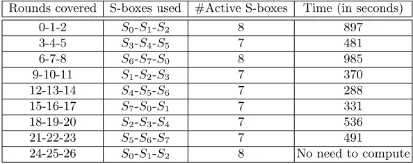
upper bound of the probability of the characteristics for round-reduced versions of a block cipher, which may lead to a tighter security bound for the full cipher. For example, using the method presented in this section, we can prove that the probability of the best characteristic covering rounds 0, 1, 2 of Serpent (using S-boxes
S0, S1 andS2) is 2−19, which is better than the result presented in Appendix B stating that the probability is upper bounded by (2−2)8= 2−16 (see Table 17 in Appendix B).
Table 5: A 4-round differential characteristic of Serpent
Rounds Input difference of the S-box layer Output difference of the S-box layer
5 (S5)
00100100000000000011001001000000 00000000000000000010000000000000 00100100000000000011000001000000 00000100000000000001001000000000 00100100000000000001001001000000 00000000000000000000001001000000 00000100000000000011000001000000 00100000000000000001001000000000
6 (S6)
10000000000000000000000000000000 00000000000000000000000000000000 00000000000000000000000000000000 00000000000000000000000000000100 10000000000000000000000000000100 10000000000000000000000000000000 00000000000000000000000000000000 00000000000000000000000000000100
7 (S7)
00000000000000000000000000000000 00000000000000000000000000000000 00000000000000000000000000000000 00000000000000000000000000000000 00000001000000000000000000000000 00000001000000000000000000000000 00000000000000000000000000000000 00000001000000000000000000000000
8 (S0)
Although the new method produces better results for a specific cipher, experimental results show that the model generated by the new technique is more difficult to solve than that generated by the method presented in Sect. 4. For example, we also apply the method to PRESENT. For 4-round PRESENT, we find its best single-key differential characteristic whose probability is 2−12 in 5 seconds, and for 8-round PRESENT, we find its best single-key differential characteristic with probability 2−32in 358675 seconds, and the corresponding characteristics are listed in Table 6 and Table 7. Compared with the models generated by the method presented in Sect. 4, the models generated by this technique involve more variables and constraints, which makes it more difficult to solve.
In practice, we can also use the new technique to find good (instead of the best) characteristic by extracting a solution from the optimizer as soon as the objective value is low enough. Although we can not make sure that the extracted solution is one of the best characteristics, this approach will reduce the time of computation significantly. Take the 8-round PRESENT as an example, the Gurobi optimizer can discover an 8-round characteristic with probability 2−32 in no more than 35008 seconds, and an 8-round characteristic with probability 2−34in no more than 18962 seconds. Note that before the Gurobi complete its computation (cost 358675 seconds in total), we can not make sure that the probability of the best characteristic is 2−32though a characteristic with this probability has already been found in just 35008 seconds.
Table 6: A 4-round single-key differential characteristic for PRESENT with the maximal possible probability
The input and output differences of the S-box layer
Rounds In Out
1 0000000000000000000000000000000000000000000000000111000000001111 0000000000000000000000000000000000000000000000000001000000000001 2 0000000000000000000000000000000000000000000000000000000000001001 0000000000000000000000000000000000000000000000000000000000000100 3 0000000000000000000000000000000100000000000000000000000000000000 0000000000000000000000000000100100000000000000000000000000000000 4 0000000100000000000000000000000000000000000000000000000100000000 0000001100000000000000000000000000000000000000000000100100000000
Table 7: An 8-round single-key differential characteristic for PRESENT with the maximal possible probability
The input and output differences of the S-box layer
Rounds In Out
1 0000000000000000000000000000000000000000000000000000000000001111 0000000000000000000000000000000000000000000000000000000000000001 2 0000000000000000000000000000000000000000000000000000000000000001 0000000000000000000000000000000000000000000000000000000000001001 3 0000000000000001000000000000000000000000000000000000000000000001 0000000000001001000000000000000000000000000000000000000000001001 4 0001000000000001000000000000000000000000000000000001000000000001 1001000000001001000000000000000000000000000000001001000000001001 5 1001000000001001000000000000000000000000000000001001000000001001 0100000000000100000000000000000000000000000000000100000000000100 6 0000000000000000100100000000100100000000000000000000000000000000 0000000000000000010000000000010000000000000000000000000000000000 7 0000000000000000000010010000000000000000000000000000000000000000 0000000000000000000001000000000000000000000000000000000000000000 8 0000000000000000000001000000000000000000000000000000000000000000 0000000000000000000001010000000000000000000000000000000000000000
6
Automatic Enumeration of (Related-key) Differential and Linear
Characteristics with Predefined Properties
By now, we are able to search for (related-key) differential or linear characteristics for a wide range of ciphers. However, just being able to obtain acharacteristicwith a small number of active S-boxes is not enough. Several works [79–81] have demonstrated that the differential attack based on one characteristic can be strengthened with multiple characteristics with the same input and output differences (the so called differential), and therefore we want to find all high probability characteristics with the same input and output differences. In the linear hull analysis, we need to find all linear characteristics with the same input and output linear masks. In the (related-key) boomerang/rectangle attack, two short differentialsα→β andγ→δare used to construct a boomerang distinguisher. By allowing β andγ to change, the probability of the constructed distinguisher can be improved. Hence, we want to find all high probability differential characteristics with a fixed input (or output) difference. In the structure attack [79], a form of differential cryptanalysis exploiting differentials with multiple input differences and a single output difference, we also need to search for characteristics sharing a same output difference. To summarize, we need to find all characteristics of some given properties according to the context, and the procedure for enumerating all characteristics covering round 1 to roundrof a cipher with some given properties is listed as follows.
Step 2. Add the constraints imposed by the given properties (concrete examples will be given in the following sections).
Step 3. Solve the model using an MILP optimizer. If a feasible solution xis found, save xto a file and update the model by adding the linear inequality l(x) to remove x from the feasible region of M; if the updated modelMis infeasible, go to Step 4. Otherwise, repeat Step 3.
Step 4. Terminate the procedure and extract all the characteristics with the given properties from the saved solutions.
In the following subsections, we show concrete applications of the above method.
6.1 Automatic (Related-key) Differential and Linear Hull Analysis
The clustering of multiple differential characteristics satisfying the same (fixed) input and output difference is referred to as the differential effect. By considering the differential effect, the computed expected differential probability (EDP) may become significantly higher than that of any differential characteristic in the differ-ential. Therefore, the probability of the differential serves to be a more accurate indication of the security of a block cipher with respect to the differential attack.
Currently available methods for searching for high probability single-key differential characteristics include the branch-and-bound approach [82], variants of Matsui’s algorithm [53, 83], and those rather dedicated methods [79, 81]. In what follows we will propose a generic and automatic method for searching for differential characteristics in a given differential in both the single-key and related-key model. The new method is not only conceptually simpler, but also easier to implement compared to existing methods.
Given an r-round differential characteristic (α0, α1, . . . , αr−1, αr), we can find all r-round differential
characteristics with the following properties: (1) the input difference is α0 and the output difference isαr,
(2) the characteristic activates at mostNA S-boxes. This can be done by the following procedure.
Step 1. Construct an MILP modelMdescribing the differential behavior of the cipher (from round 1 to round r) according to Sect. 4.
Step 2. Add the constraints describing that the input difference must beα0 and the output difference must beαr(these constraints are simple equations fixing the input and output bit-level differences), and add
the constraintP
jSj≤NA, where theSj’s are variables marking the activities of the S-boxes involved.
Step 3. Solve the model using an MILP optimizer. If a feasible solution xis found, save xto a file and update the model by adding the linear inequality l(x) to remove x from the feasible region of M; if the updated modelMis infeasible, go to Step 4. Otherwise, repeat Step 3.
Step 4. Terminate the procedure and extract all the differential characteristics in the differential with at mostNA active S-boxes from the saved solutions.
Differential Analysis of SIMON and LBlock. SIMON [84] is a family of lightweight block ciphers designed by the U.S. National Security Agency (NSA). The design of SIMONnb/nK is a Feistel scheme with
a block size of nb bits and key size of nK bits. The bitwise AND operation is the only nonlinear operation
of SIMONnb/nK. For a detailed description of SIMON and existing attacks on it, we refer the reader to [53,
58, 59, 82, 84–87].
By treating the AND (F2×F2→F2) operation as a 2×1 S-box, we apply our method to SIMON in the
single-key model. In our MILP models we treat the input bits of the AND operation asindependent input bits, and the dependencies of the input bits to the AND operation are not considered. Therefore, the characteristic obtained by our method is not guaranteed to be valid for SIMON (other ciphers do not have this problem). Hence, every time after the Gurobi optimizer outputs a good solution (characteristic), we check its validity and compute its probability by the method presented in [53].
We find a 16-round single-key differential characteristic for SIMON48 with probability 2−50 (see Table 8). Then we compute the probability of the differential with its input and output differences fixed to the values given in Table 8 with the method presented in this section. To be more specific, we search for all characteristics with probabilitypsuch that 2−60≤p≤2−50in this differential, and the distribution of these characteristics is given in Table 9, from which we can deduce that the probability of this differential is greater than 2−44.65. To the best of our knowledge, this is the first published single-key differential covering more than 15 rounds of SIMON48.
Table 8: A single-key differential characteristic of 16-round SIMON48 with probability 2−50.
Rounds The input differences
0 (Input) 100000000000000000000000 001000100000000010000010 1 001000100000000000000000 100000000000000000000000 2 000010000000000000000000 001000100000000000000000 3 000000100000000000000000 000010000000000000000000 4 000000000000000000000000 000000100000000000000000 5 000000100000000000000000 000000000000000000000000 6 000010000000000000000010 000000100000000000000000 7 001000100000001000000000 000010000000000000000010 8 100000100000100000100000 001000100000001000000000 9 001000100000001000000000 100000100000100000100000 10 000010000000000000000010 001000100000001000000000 11 000000100000000000000000 000010000000000000000010 12 000000000000000000000000 000000100000000000000000 13 000000100000000000000000 000000000000000000000000 14 000010000000000000000000 000000100000000000000000 15 001000100000000000000000 000010000000000000000000 16 (Output)100000000000000000000000 001000100000000000000000
Table 9: The distribution of the characteristics of SIMON48 in the differential specified by the input and output differences given in Table 8. The invalid characteristics is due to the special property of the dependent inputs of the AND operations in SIMON, and we refer the reader to [51, 53] for more information.
Probability 2−502−512−522−532−542−552−562−57 2−58 2−59 2−60 Invalid #Characteristics 1 6 15 46 100 114 379 685 953 913 724 3568
Table 10: A single-key differential characteristic of the 21-round SIMON64 with probability 2−70.
Rounds The input differences
0 (Input) 00000000000010000000000000000000 00000000001000100010000000000000 1 00000000000000100010000000000000 00000000000010000000000000000000 2 00000000000000001000000000000000 00000000000000100010000000000000 3 00000000000000000010000000000000 00000000000000001000000000000000 4 00000000000000000000000000000000 00000000000000000010000000000000 5 00000000000000000010000000000000 00000000000000000000000000000000 6 00000000000000001000000000000000 00000000000000000010000000000000 7 00000000000000100010000000000000 00000000000000001000000000000000 8 00000000000010000000000000000000 00000000000000100010000000000000 9 00000000001000100010000000000000 00000000000010000000000000000000 10 00000000100000001000000000000000 00000000001000100010000000000000 11 00000010001000000010000000000000 00000000100000001000000000000000 12 00001000011000000000000000000000 00000010001000000010000000000000 13 00000011001000000010000000000000 00001000011000000000000000000000 14 00000000100000001000000000000000 00000011001000000010000000000000 15 00000000001000100010000000000000 00000000100000001000000000000000 16 00000000000010000000000000000000 00000000001000100010000000000000 17 00000000000000100010000000000000 00000000000010000000000000000000 18 00000000000000001000000000000000 00000000000000100010000000000000 19 00000000000000000010000000000000 00000000000000001000000000000000 20 00000000000000000000000000000000 00000000000000000010000000000000 21 (Output)00000000000000000010000000000000 00000000000000000000000000000000
Table 11: The distribution of the characteristics of SIMON64 in the differential specified by the input and output differences given in Table 10.
By adding the constraints that the input and output differences are fixed to be the values suggested in Table 10, we search for all characteristics in this differential with probabilitypsuch that 2−79≤p≤2−70. We obtain 159554 characteristics (including 19942 invalid ones) in total with varying probability. The details of the distribution of these characteristics are given in Table 11, from which we can deduce that the probability of the differential for the 21-round SIMON64 is greater than 2−60.21. Note that the probability of the best previously published 21-round differential for SIMON64 is 2−60.53. By extending one more round of this differential, we obtain a 22-round single-key differential characteristic for SIMON64 with probability at least 2−62.21, which is the first published single-key differential characteristic covering more than 21 rounds of SIMON64. Note that the 21-round characteristic presented in [53] can not be simply extended to obtain a 22-round characteristic with probability less than 2−64, since the Hamming weight of its output is higher and extending one more round will decrease the probability significantly. The differentials presented in this paper for SIMON can be used to produce the best differential attacks on SIMON48 and SIMON64 with Wang et al.’s technique [58].
We also apply the method to LBlock, and we find a 16-round standard (non truncated) related-key
differentialwith probability 2−55.64, which is even better than the previously published besttruncated related-key differential for the 16-round LBlock whose probability is about 2−59[57]. The results are given in Appendix D.
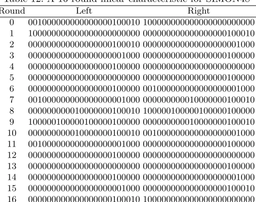
Linear (Hull) Analysis of SIMON48. For the sake of completeness, we also present an example on SIMON48 demonstrating that our method is also applicable inlinear hullanalysis, and this part can be safely skipped by the readers since there is no essential difference between the two methods for differential and linear hull analysis. Alinear hull, first announced by Nyberget al.in [88], is a collection of linear characteristics with a certain (fixed) input and output masks. It is the counterpart to differentialsin differential cryptanalysis, and there are a lot of works (e.g.[89–95]) studying the linear hull effect.
Using the MILP technique, we find a 16-round linear characteristic with bias 2−26 (see Table 12). By considering multiple linear approximations with the same input and output masks specified in Table 12, we obtain 394271 linear characteristics where 16767 characteristics are valid, which lead to a linear hull with
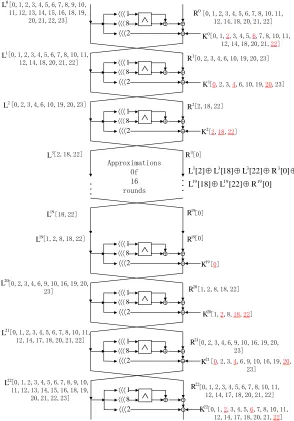
potential2−44.92. Using Matsui’s Algorithm 2 [96], we can attack 23-round SIMON48/96 by adding 3 rounds at the top and 4 rounds at the bottom of the linear hull (see Fig. 1 in Appendix E). Note that the subkey bits without underscore are secret bits to be guessed in the attack. To the best of our knowledge, there is no published linear attack on SIMON48/96 which can cover 23 rounds of SIMON48/96.
Table 12: A 16-round linear characteristic for SIMON48
Round Left Right
6.2 Automatic Truncated (Related-key) Differential Analysis
In basic truncated differential analysis, the fixed output differenceβ of a differentialα→β is truncated to be a bit string with some specific bits allowed to be any valued in{0,1}. With this relaxation, the probability of the truncated differential can be increased. Truncated differential is a very useful tool in cryptanalysis and several ciphers which are secure against standard differential attack are vulnerable to truncated differential attack.
We now present an automatic method for enumerating all high probability (related-key) differential char-acteristics in a given truncated (related-key) differential.
Step 1. Construct an MILP modelMdescribing the differential behavior of the cipher (from round 1 to round r) according to Sect. 4.
Step 2. For a given truncated differentialα0→αrwhereαr= (αr,0, . . . , αr,n−1) and
αj0= 0,· · · , αjsr = 0
αjsr+1= 1,· · ·, αjst = 1
αjst+1=∗,· · ·, αjn−1 =∗,
(7)
add the system of equations
αj0 = 0,· · ·, αjsr = 0
αjsr+1 = 1,· · · , αjst = 1
(8)
and the constraintP
jSj ≤NA into the modelM, where theSj’s are the variables marking the activities of
the S-boxes involved.
Step 3. Solve the model using an MILP optimizer. If a feasible solution xis found, save xto a file and update the model by adding the linear inequality l(x) to remove x from the feasible region of M; if the updated modelMis infeasible, go to Step 4. Otherwise, repeat Step 3.
Step 4. Terminate the procedure and extract all the differential characteristics in the given truncated differential with at mostNA active S-boxes from the saved solutions.
We apply the above method to DESL. Firstly, we find a related-key differential characteristic for the 9-round DESL, and the results are given in Table 13 and Table 14.
Table 13: A 9-round related-key differential characteristic for DESL (characteristic in the encryption process)
Rounds Left Right
0 00000000000000010000000000000000 00000000010000000000000000000000 1 00000000010000000000000000000000 00000000000000000000000000000000 2 00000000000000000000000000000000 00000000010000000000000000000000 3 00000000010000000000000000000000 00000100000000000000000000000000 4 00000100000000000000000000000000 00000000010000000100000000000000 5 00000000010000000100000000000000 00100000000000000000000110000000 6 00100000000000000000000110000000 00000010110000000100000000000000 7 00000010110000000100000000000000 00000000000001000000000000000000 8 00000000000001000000000000000000 00000010100000000100000000000000 9 00000010100000000100000000000000 00100100000010000000000000000000
Then, we truncate the output difference (the input difference of the 10th round) to be
00000010100000000100000000000000 0**00*0*0000**0*0*00000**00*0*00
and we try to find all related-key differential characteristic with at most 21 active S-boxes in this truncated key differential. Finally, we find 14700 characteristics in total leading to a 9-round truncated related-key differential for DESL with probability 2−34.06.
6.3 Automatic Construction of (Related-key) Boomerang/Rectangle Distinguishers
Table 14: A 9-round related-key differential characteristic for DESL (characteristic in the key schedule algo-rithm)
Rounds The differences in the key register
1 000000000000000010000000000000000000000000000000 2 000000000000000000000000000000000000000000000000 3 000000000000100000000000000000000000000000000000 4 000000000010000000000000000000000000000000000000 5 000000000000010000000000000000000000000000000000 6 010000000000000000000000000000000000000000000000 7 000000001000000000000000000000000000000000000000 8 000000000000000000000010000000000000000000000000 9 000000000000001000000000000000000000000000000000
block cipher which can be described asE=E1◦E0, such that for E0there exists a differentialα→β with probability p, and forE1 there exists a differentialγ→δwith probabilityq.
In the rectangle distinguisher, the attacker constructs quartets of plaintexts of the form (P1, P2, P3, P4) such that P1⊕P2 = P3⊕P4 =α. A quartet is said to be a right quartet if the following conditions are satisfied:
1. E0(P1)⊕E0(P2) =E0(P3)⊕E0(P4) =β; 2. E0(P1)⊕E0(P3) =γ (orE0(P2)⊕E0(P4) =γ); 3. C1⊕C3=C2⊕C4=δ.
It can be shown that the probability of a quartet to be right is approximately 2−n(pq)2. The above process can be used to distinguish E from a random permutation if (pq)2 >2−n, since for a random permutation,
the probability ofC1⊕C3=C2⊕C4=δ is 2−2n.
It is suggested in [97] that the attack can be mounted for all possibleβ’s and γ’s to improve the attack. Therefore the rectangle process can be employed to distinguishEfrom a random permutation if (ˆpqˆ)2>2−n, where
ˆ
p=
s X
β
P r2[α→β] and qˆ=
s X
γ
P r2[γ→δ]
In some cases, this improvement reduces the complexity for the rectangle attack significantly. In practice, ˆ
pis computed as follows. Firstly, the attacker finds a differential (or differential characteristic)α→β forE0 with probabilityp0. Then he or she tries to find all high probability differentials with input differenceα. For example, if he or she obtainnj differential (characteristics) with probabilitypj, then ˆpcan be approximated
by qP
jnjpj2. Similar situation is also encountered in the so called structure attack [79], in which the
attacker needs to find high probability differentials sharing the same output difference. We now show that such tasks can be accomplished automatically with an MILP technique, and the procedure is presented as follows.
Step 1. Construct an MILP modelMdescribing the differential behavior ofE0 according to Sect. 4. Step 2. Add the constraints describing that the input difference must beα0 (these constraints are simple equations fixing the input bit-level differences), and add the constraint P
jSj ≤ NA, where the Sj’s are
variables marking the activities of the S-boxes involved andNA is chosen by the attacker to make sure that
the probabilities of the characteristics found are not too small.
Step 3. Solve the model using an MILP optimizer. If a feasible solution xis found, save xto a file and update the model by adding the linear inequality l(x) to remove x from the feasible region of M; if the updated modelMis infeasible, go to Step 4. Otherwise, repeat Step 3.
Step 4. Terminate the procedure and extract all the differential characteristics in the differential with at mostNA active S-boxes from the saved solutions, and compute ˆpby the above method.
to find all characteristics with at most 9 active S-boxes whose input difference to the S-box of the first round is
0010000000000000000000000000000000000000000000000000000000000000.
Finally, we obtain totally 1028 characteristics. There are 4 characteristics with probability 2−11, 128 char-acteristics with probability 2−19, 256 characteristics with probability 2−20, 512 characteristics with probability 2−21, and 128 characteristics with probability 2−22. Hence the overall probability ˆpforE
0 is approximately
p
4×(2−11)2+ 128×(2−19)2+ 256×(2−20)2+ 512×(2−21)2+ 128×(2−22)2≈2−10.
Table 15: A 7-round related-key characteristic for PRESENT-128 (characteristic in the encryption process)
The input and output differences of the S-box layer
Rounds In Out
1 0010000000000000000000000000000000000000000000000000000000000000 0101000000000000000000000000000000000000000000000000000000000000 2 0000000000000000000000000000000000000000000000000000000000000000 0000000000000000000000000000000000000000000000000000000000000000 3 0000000000000000000000000001000000000000000000000000000000000000 0000000000000000000000001101000000000000000000000000000000000000 4 0000001000000000000000000000000000000000000000000000000000000000 0000001100000000000000000000000000000000000000000000000000000000 5 0000000000000000000000000000000000000000000000000100000000000000 0000000000000000000000000000000000000000000000000101000000000000 6 0000000000000000000000000000000000000000000000000000000000000000 0000000000000000000000000000000000000000000000000000000000000000 7 0000000000000000000000000000000000000001000000000000000000000000 0000000000000000000000000000000000000111000000000000000000000000
Table 16: A 7-round related-key characteristic for PRESENT-128 (characteristic in the key schedule algo-rithm)
Rounds The differences in the key register
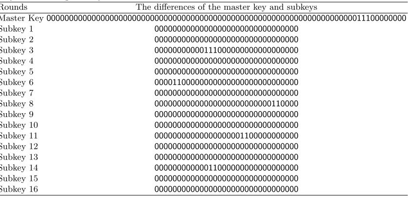
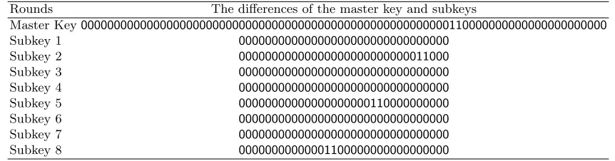
0 (Master Key) 00000000000000000000010000000000000000000000000000000000000000000000000000000100000000000000000000000000000001000000000000000000 1 00000000000000001000000000000000000000000000000010000000000000000000000000000000000000001000000000000000000000000000000000000000 2 00000000000000000000000000010000000000000000000000000000000000000000000000000000000100000000000000000000000000000001000000000000 3 00000000000000000000001000000000000000000000000000000010000000000000000000000000000000000000001000000000000000000000000000000000 4 00000000000000000000000000000000010000000000000000000000000000000000000000000000000000000100000000000000000000000000000001000000 5 00000000000000000000000000001000000000000000000000000000000010000000000000000000000000000000000000001000000000000000000000000000 6 00000000000000000000000000000000000000010000000000000000000000000000000000000000000000000000000100000000000000000000000000000001 7 00000000000000000000000000000000001000000000000000000000000000000010000000000000000000000000000000000000001000000000000000000000 8 00000101000000000000000000000000000000000000010000000000000000000000000000000000000000000000000000000100000000000000000000000000
Using this result and the related-key differential characteristic coveringE1 (specified in [98]) with proba-bility ˆq≈2−12 presented in [98], we can produce an improved related-key rectangle attack on the 17-round PRESENT-128 using the same method presented in [98].
Using the same method, we also obtain an improved related-key boomerang distinguisher for LBlock, and the result is given in Appendix F.
7
Limitations of the Method
The method presented in this paper has some limitations which we are not able to overcome. Firstly, this method is not practically applicable to evaluate the security of ARX/LRX constructions. Although we can treat the addition mod 2nas a 2n×nS-box and compute the convex hull of all its differential patterns, this
is impractical for real ARX ciphers wherenis typically at least 16. For practical tools which can be applied to ARX/LRX constructions, we refer the reader to [83, 99–103]. For ARX/LRX constructions, we think the approaches proposed by Mouhaet al.[99], Aumassonet al. [103] and K¨olbl [104] are promising.
Secondly, the method is not exact for all ciphers. In the case of SIMON, we do not know how to construct an MILP model whose feasible region contains no invalid characteristics due to its dependent inputs. A method which can be used to construct an exact model for SIMON will make the analysis of SIMON much more convenient.
Finally, it seems that the technique can be applied mostly to lightweight ciphers since the solution of a MILP model with thousands of variables and constrains is really difficult. Therefore, further investigation of how to solve such models efficiently is of great importance.