Lock-free GaussSieve for Linear Speedups in
Parallel High Performance SVP Calculation
Artur Mariano
Institute for Scientific Computing Technische Universit¨at DarmstadtDarmstadt, Germany [email protected]
Shahar Timnat
Department of Computer Science Technion - Israel Institute of TechnologyHaifa, Israel [email protected]
Christian Bischof
Institute for Scientific Computing Technische Universit¨at DarmstadtDarmstadt, Germany [email protected]
Abstract
Lattice-based cryptography became a hot-topic in the past years be-cause it seems to be quantum immune, i.e., resistant to attacks op-erated with quantum computers. The security of lattice-based cryp-tosystems is determined by the hardness of certain lattice problems, such as the Shortest Vector Problem (SVP). Thus, it is of prime im-portance to study how efficiently SVP-solvers can be implemented. This paper presents a parallel shared-memory implementation of the GaussSieve algorithm, a well known SVP-solver. Our imple-mentation achieves almost linear and linear speedups with up to 64 cores, depending on the tested scenario, and delivers better sequen-tial performance than any other disclosed GaussSieve implementa-tion. In this paper, we show that it is possible to implement a highly scalable version of GaussSieve on multi-core CPU-chips. The key features of our implementation are a lock-free singly linked list, and hand-tuned, vectorized code. Additionally, we propose an al-gorithmic optimization that leads to faster convergence.
Keywords GaussSieve, SVP, parallel, mul1ti-core CPU, lock-free
1.
Introduction
Cryptography is mainly used to protect information that is sent over an insecure channel. In 1996, Ajtai found out that some lattice prob-lems have interesting properties for cryptography, such as average-case hardness [1]. Cryptosystems based on lattices are said to fall within the realm oflattice-based cryptography, a rapidly expanding field since Ajtai’s discoveries on lattice problems. Lattices are dis-crete subgroups of them-dimensional Euclidean spaceRm, with
a strong periodicity property. A latticeLgenerated by a basisB, a set of linearly independent vectorsb1,...,bninRm, is denoted by:
L(B) ={x∈Rm:x=
n
X
i=1
uibi,u∈Zn} (1)
wherenis the rankof the lattice. When n = m, the lattice is said to be offull rank. When mis at least 2, each lattice has infinitely many different bases.
Lattice-based cryptography is particularly attractive since lattice-based cryptosystems are believed to be quantum immune, i.e., re-sistant to attacks operated with quantum computers. Lattice-based cryptosystems can only be broken when specific lattice problems can be solved in a timely manner. As the security of these sys-tems is estimated based on the performance of the algorithms that solve their underlying problems, highly optimized and parallelized solvers are needed to realistic estimations. One of the underlying problems in lattice-based crypto-systems is to find the shortest vec-tor in a given lattice, a problem referred to as the Shortest Vecvec-tor Problem (SVP). The SVP consists in finding the nonzero vector vof a given latticeL, whose normkvkis the smallest among the norms of all nonzero vectors in the latticeLand is denoted by λ1(L). The problem can be stated for every norm; In this paper, we address the Euclidean norm, the most common in this context. An algorithm that solves the SVP is called aSVP-solver.
SVP-solvers work faster on reduced lattice bases, i.e. lattice bases with short, nearly orthogonal vectors. The main algorithms that can be used to reduce lattices are the Lenstra-Lenstra-Lov´asz (LLL) and the Block Korkine Zolotarev (BKZ) algorithms (cf. [8]). LLL sparked a new era of research on lattice basis reduction. Lattice basis reduction algorithms can be used to solve approximate solutions of the SVP. In fact, for lattices in two dimensions, the LLL algorithm solves the SVP exactly. Lattice basis reduction algorithms are widely used in many fields and in cryptanalysis, including in different types of cryptography, such as knapsack cryptosystems and special settings of RSA. In this paper, we use BKZ to pre-reduce the lattices in which we solve the SVP on.
There are three main classes of SVP-solvers: sieving algo-rithms, enumeration algorithms and algorithms based on the Voronoi cell of a lattice (see [8] for a comprehensive overview). Sieving al-gorithms were introduced in 2001, via the AKS algorithm [2], and extended in 2010, with algorithms that improve the complexity of AKS [11]. An asymptotic better variant of the AKS algorithm, called ListSieve, as well as its efficient heuristic GaussSieve, were presented by Micciancio et al. [11]. While ListSieve was consid-ered of low practicability, the authors did also present an efficient heuristic of ListSieve, called GaussSieve. A theoretical improve-ment of ListSieve was presented by Pujol et al. [16]. Recently, a three-level sieving heuristic, with better time and space complexity than ListSieve, was proposed [18]. However, it is still unclear if it can perform better than GaussSieve, because neither there is a prac-tical implementation of it nor is the time complexity of GaussSieve known.
iteration to be given as input. This is a major problem because the optimal value for this parameter is not known upfront, and sub-optimal values increase the time that the algorithm takes to con-verge. In Section 3.2 we overview both implementations in detail.
At this point in time, the fastest probabilistic approach to solve the SVP in practice, in terms of running time, seems to be enumer-ation solvers with extreme pruning. However, sieving algorithms are still interesting because (1) they are asymptotically better than enumeration (2O(n)
vs.2O(nlogn)
), (2) they can take more advan-tage of specific lattices, such as ideal lattices, than enumeration al-gorithms (see [15], Section 6.1) and (3) some advances in sieving algorithms have been published during the last years and it is ex-pected that further optimizations will be proposed in the next years. For instance, this paper proposes one algorithmic optimization that enables GaussSieve to converge faster.
Our contribution is three-fold. In addition to the aforementioned algorithmic optimization of the GaussSieve algorithm, we present a parallel, scalable multi-core implementation that slightly relaxes the properties of GaussSieve, with negligible impact on the time for convergence. Our implementation delivers high levels of perfor-mance due to hand-tuned and vectorized code. Finally, we propose an extension to the lock-free list proposed in [5], which is used as the core of our implementation.
This paper is organized as follows. Section 2.1 provides rele-vant notation and recaps some definitions, and Section 2.3 explains the GaussSieve algorithm. In Section 3, we overview related work, both concerning SVP-solvers in general, and parallel implementa-tions of the GaussSieve algorithm in particular. Section 4 explains our approach in detail and the implemented optimizations. Sec-tion 5 shows how our implementaSec-tion performs and compares with other parallel implementations of GaussSieve. Finally, Section 6 concludes the paper and provides some future lines of research.
2.
Preliminaries
2.1 Notation and definitions
The Euclidean norm of a vector is the distance spanned from the origin of the lattice to the point given by the vector v, i.e. kvk=pPni=1v2
i, whereviis the ithcoordinate ofv. We use the
termzero vectorfor vectors whose norm is zero, i.e., the origin of the lattice. Vectors and matrices are written in bold face, vectors are written in lower-case, and matrices in upper-case, as in vectorv and matrixM. The dot product of two vectorsvandpis denoted by hv,pi. The latticeLgenerated by a basisBis denoted byL(B). We now give two important definitions in the context of the GaussSieve algorithm:
Definition 1 - Gauss-Reduced:Two vectorspandv∈ L(B)
are said to be Gauss-reduced (with respect to each other) when min(kp±vk)≥max(kpk,kvk) holds true. A simple routine to re-duce two vectorspandvwas presented in [11], and is referred to as theReducekernel. When this routine is invoked bi-directionally, i.e.,Reduce(p,v) andReduce(v,p),pandvbecome Gauss-reduced.
Definition 2 - Pairwise-reduced:A set or a listLof vectors is pairwise-reduced, i.e., all its elements are pairwise-reduced, when every pair (p,v)∀p,v∈L, is Gauss-reduced.
We also recall the definitions of speedupSpand efficiencyEp,
presented in Equation 2. and 3, respectively.
Sp=
T1
Tp
, (2)
whereTpis the program’s execution time withpprocessors.
Ep=
Sp
p = T1
pTp
(3)
2.2 The Shortest Vector Problem
Virtually every lattice problem has to do withdistances. In partic-ular, the SVP consists in finding the non-zero vectorvof a given latticeL, whose normkvkis the smallest among the norms of all nonzero vectors in the latticeL. This norm is usually denoted by λ1(L)or simplyλ1, if it is clear what lattice is concerned. As a
result, the SVP can formally be defined as the computation of a vectorv∈ L(B)\ {0}wherekvk=λ1(L(B)). The problem can be stated for every norm; In this paper, we address the Euclidean norm, the most common in this context.
The picture of the best SVP-solvers has been changing during the last decade. In particular, enumeration and sieving have been two concurrent approaches, competing for the position of the best SVP-solver. Sieving algorithms were first thought to be impracti-cal, until the AKS algorithm was proven to be practiimpracti-cal, in 2008 [13], even though still uncompetitive with enumeration routines. In 2010, Micciancio et al. presented GaussSieve, the first sieving heuristic that outperformed enumeration routines [11]. However, in the same year, Gama et al. proposed theextreme pruning ap-proach for enumeration algorithms [4], which drove GaussSieve, and consequently sieving algorithms, out of the podium. This ap-proach reduces the probability of enumeration algorithms to find the shortest vector of a lattice, but it reduces their running time by a much higher factor. The method shuffles the basis and runs the extreme pruned enumeration on it, repeating the process until the shortest vector is found. In practice, enumeration with extreme pruning becomes probabilistic and a probabilistic stopping crite-rion, as in sieving algorithms, must be used instead.
Although enumeration algorithms became the main line of re-search in lattice-based cryptanalysis, several studies on sieving al-gorithms were still published since 2010 [6, 9, 12, 14, 15, 17, 18]. As mentioned before, sieving algorithms are still of prime impor-tance, because they can be adapted to take advantage of special lattice structures, in contrast to enumeration algorithms [15]. Siev-ing algorithms might have attracted less attention than enumera-tion algorithms also because they have been thought to be difficult to parallelize. In particular, Fitzpatrick et al. presented several im-provements to GaussSieve, which offer considerable speedups in practice [3]. From those, we highlight an approach that enables to estimate the angle between two vectors, which can be implemented very efficiently with vectorized routines. Mariano et al. also showed very recently that ListSieve, an algorithm categorized as impracti-cal, is actually practiimpracti-cal, especially in massively parallel architec-tures [10].
In this paper, we show that GaussSieve can, in fact, be paral-lelized and implemented in a very effective manner, by slightly relaxing its properties. We hope that this might help to shift the attention of the community towards sieving algorithms.
2.3 The GaussSieve algorithm [11]
The algorithm is based on sampling lattice vectors and building a listLof shorter (of smaller norm) and shorter vectors. The sampled vectors, referred to assamples, undergo a two-stage reduction pro-cess. For each samplev, this process is based on (1) reducingv, when possible, with every vectorpinL, thus obtainingv’, and (2) reducing every possible vectorpinLwithv’. As a result, the listL will only hold Gauss-reduced vectors. The algorithm also employs a stackSto keep vectors that are temporarily removed fromL.
process is not executed and the number of collisions is incremented. Otherwise, stage (1) does not generate a zero vector but av’instead, and stage (2) is executed. In stage (2), the algorithm checks if any vectorl∈Lcan be reduced againstv’. All such vectors are temporarily removed fromL, reduced againstv’and pushed to the stackS. At the beginning of each iteration, the algorithm checks ifScontains any vector. If this holds, a vector fromSis used as a sample, otherwise a new vector is sampled.
This is iteratively executed until a certain stopping criterion, K ≥c, whereKis the number of collisions, is met. By then, the shortest vector is expected to be inL.cis usually set in the formc=
α×mls+β, wheremlsis the maximum size ofLup to that point. The workflow of the algorithm is shown in Algorithm 1. Although the samples can be generated by any algorithm, they are typically generated with Klein’s algorithm, as in [7]. Klein’s algorithm has very good theoretical guarantees, and it samples vectors according to a distribution that is statistically close to Gaussian (the variance is arbitrary). This is particularly desirable for GaussSieve, since no direction in space is privileged, and collisions are mostly generated only after the shortest vector is found [13, 14].
The algorithm is not trivially parallelizable. At a fine-grained level, while stage (1) of the reduction process is easily paralleliz-able, phase (2) is not. At a course- grained level, the listLwould be read and written by multiple threads, which is not safe unless some sort of synchronization is used. In Section 3.2, we describe the approaches that were followed to parallelize the algorithm. Our approach is based on parallelizing the algorithm at a course-grained level, employing a scalable, thread-safe mechanism that permits the use ofLwith minimal synchronization.
Algorithm 1:GaussSieve algorithm Input:BasisB;
Init:L← {}, S← {}, K←0
whileK < cdo ifS is not emptythen
v←S.pop(); else
v←SampleKlein();
v←GaussReduce(v,L, S); ifkvk==0then
K←K+ 1;
else
L←L∪ {v};
functionGaussReduce(p,L,S) while∃vi∈L:kvik ≤ kpk∧
kp−vik ≤ kpkdo
p←p−vi;
end
ifkpk==0then return p;
while∃vi∈L:kvik>kpk∧
kvi−pk ≤ kvikdo
L←L\ {vi};
S.push(vi−p);
return p;
3.
Related Work
In this section we overview the available implementations of SVP-solvers and the parallel implementations of GaussSieve.
3.1 Sequential SVP-solvers
There are various implementations of SVP-solvers. The fplll1 li-brary implements several algorithms on lattices, mainly relying on floating-point computations. As far as the SVP is concerned, it includes a floating-point implementation of the Kannan-Fincke-Pohst algorithm, here on referred to asfplll’s svp. This is currently considered the most efficient sequential available implementation of an enumeration routine without pruning. Panagiotis Voulgaris published a C++ sequential implementation2 of GaussSieve, here
1http://perso.ens-lyon.fr/damien.stehle/fplll/ 2http://cseweb.ucsd.edu/˜pvoulgar/impl.html
on referred to as the gsievelibrary, used in the experiments of the original GaussSieve paper [11]. In this paper, we compare the performance of our sequential implementation with both. To the best of our knowledge, there are no available implementations of enumeration-based routines with extreme pruning.
3.2 Parallel implementations of GaussSieve
In 2011, Milde et al. published a first parallel version of the GaussSieve algorithm [12]. The implementation consists of a ring structure connecting several instances of GaussSieve, each con-taining alocal list Land a private stackS. Each instance is then executed by a thread, which samples vectors, one by one, reduces them against its local listL, and hands them out to the ring structure. Each vector floats around the ring structure, by means of buffers, where it is picked by every thread, and reduced against the local list therein. When the vector returns to the thread that released it, it is added to the local list of that thread.
In the results shown in [12], the implementation does not scale well for more than 4 threads (the efficiency is≥85% only for 4 or fewer threads), because the number of iterations required for con-vergence increases with the number of threads. This happens be-cause the local lists progressively hold more and more vectors that are not Gauss-reduced with all the other vectors in the remaining lists: if any vectorvof a threadipasses by the local list of threadt, between the release of a vectorp, by threadt, and its commitment to the local list of threadt,vandpwill never be reduced against each other. The bigger the number of threads running on the sys-tem, the more often this case occurs and therefore the greater the number of iterations required for convergence.
In 2013, Ishiguro et al. proposed another parallel version of GaussSieve [6], for shared and distributed memory systems, with better scalability on shared memory systems3, at least up to 8 threads. Their implementation is based on the following property of union of pairwise-reduced sets: if two setsAandBare pairwise-reduced and every pair of vectors (a,b) is Gauss-reduced,∀a∈
A,b∈B, thenA∪Bis also pairwise-reduced.
The algorithm sets up a listVwithrsamples, withrprovided as input, and applies a 3-stage reduction process. In stage (1), the sample vectors inVare reduced against the vectors inL, identically to the original GaussSieve algorithm, but in parallel. Every vector that is modified in this process is added to the stackS, otherwise it is moved to aV’list, whose elements can not be further reduced with any element inL. In stage (2), the original vectors inV’ are reduced against one another, in parallel. We emphasize that the reduced vectors are the original vectors inV’, otherwise this would represent a dependency. As a result, the vectors inV’must be copied to a separate variable before the reduction against other vectors. The modified vectors are moved onto the stackS, whereas the unmodified vectors are moved to a listV”. In stage (3), each thread reduces a part ofLagainst the elements inV”. Again, if any vector is changed in the reduction process, it is added to the stack S, otherwise it is added toL’. LikeV”,L’is also pairwise-reduced. Once this 3-stage process is concluded,L’andV”are merged to create the new listLand the listVis filled up with the vectors that are inS(if they do not totalrvectors, more are generated and added toV). This whole process re-starts until the number of collisionsK reaches a certain thresholdc. However, ifKreachescin the midst of one iteration, that whole iteration, which containsrsamples, is still fully executed. The original algorithm, on the contrary, stops as soon as the number of samples reaches the desired boundaryc.
This approach has two major drawbacks. While it exposes par-allelism and permits good scalability on shared memory systems, (1) the use ofrsamples increases the computation that is necessary
for convergence and (2) the optimal value ofris never known up-front. In fact, there is a close relation between how optimalris and the runtime of the algorithm (see Figure 3(a) in [6]). Additionally, the optimal value for this parameter varies, very likely, from lattice to lattice and from dimension to dimension. Therefore,rmust be chosen on the basis of empirical tests, but there is no point in solv-ing the SVP on the same lattice twice. We can therefore assume that a non-optimal parameter will always be chosen in first place.
There are also some implementation details that are not dis-cussed in the paper, and it is unclear how they are solved and how much overhead they cause in the implementation. For example, in the three stages of the reduction process, several vectors are moved to the stackS, which represents a dependency. In Algorithm 4, in the Appendix of [6], only three kernels, which exclude the inser-tions inS, are run in parallel. This means that that insertions inS are sequential, which limits scalability.
Our implementation attains much better scalability figures than in [12] and better performance than the results reported in [6], whose code is undisclosed, thereby preventing us from carrying out thorough comparisons.
4.
Lock-free GaussSieve Implementation
The root of the main problems in the implementations described in Section 3.2 is the distribution of the original list L. In [12], vectors fluctuate between a number of different data-structures and might fail at encounter one another during the reduction process. In contrast to the previously described implementations, we keep the vectors in a central listL, safely accessible by every thread concurrently. Unlike scenarios with multiple local lists, as in [12], vectors are likely to see one another during the reduction process, because they are physically close to one another. In particular, not only two vectorsvandpare likely to encounter each other during the reduction process, but reduced versions of these vectors are also likely to encounter one another, as discussed in Section 4.2. This approach is also better than [6], because (1) it does not need extra parameters for which the optimal values are not known upfront and (2) it stops as soon as the threshold of collisions is reached.
Our implementation is written in C++, uses OpenMP to man-age a team of threads and uses gsieve’s implementation of Klein’s. It sets up a shared lock-free listL, which is an enhanced version of Harris’s linked list [5]. Each thread executes the original workflow of the algorithm: they sample a vectorv, reduce it against every vec-torpinL, obtainingv’, and reduce every vectorpinLagainstv’. Each thread has also a private stackS, werep’=Reduce(p,v’) is moved onto, wheneverp’6=p. Our lock-free implementation relies on the compare-and-swap atomic primitive for synchronization.
4.1 Enhanced lock-free list
We implemented the lock-free linked list described in [5], with some modifications and extensions. Each node in the list represents a vector, and includes an arraydata[N], which represents the co-ordinates of the vectors, a longnorm, which holds the norm of the vectors, and a pointerNode *nextto the next element in the list.
Nis the dimension of the lattice.
struct Node{
DATATYPE attribute ((aligned(8))) data[DIMENSION];
long norm; Node *next;
}
datais an array of eitherints orshorts. The list is ordered by increasing norm, similarly tokeyin [5]. For the atomics, we used compiler built-in functions.
Vectors in the shared list should not be directly modified, since if two threads concurrently modify the same vector the result could be erroneous. If a thread wishes to modify a vector, it should instead remove it from the list and insert a modified version of it. This requires a slight change in theReducefunction of thegsievelibrary. This function tests ifpshould be reduced againstv, changingpif the test holds true, removing it fromLafterwards. We splitReduce into two other functions,testReduce andeReduce, thus ensuring that vectors are never modified while inL.
testReducetests ifpshould be reduced againstv. It does so by computingdot=hp,viand then testing whether(abs(2∗dot)≤ kvk). If the result is true, thenvis removed fromL, and copied to a different variable. This copy ofvis updated usingeReduce, and pushed onto the stackS(the private stack of the relevant thread). If the result is false,eReduceis not called. To avoid performance losses, the variabledotis passed by reference totestReduce, so it can be reused ineReducewithout any recalculation.
As for stage (1) in the GaussSieve function, a sample vectorp is reduced against all the vectorsl∈Lsuch thatklk ≥ kpk. This is a straightforward process, because all the threads can read the list concurrently (as mentioned, elements are never written while inL), and therefore reduce their own samples. After this process,pis to be inserted inL, such thatLremains ordered.
Both theinsertandremovemethods in Harris’s linked list use an internal search method, which searches for a given key (a vector norm in our case) from the beginning of the list. However, in the lock-free GaussSieve implementation, it is superfluous to search for the desired norm from the beginning ofL. If during the traversal a vectorpthat should be reduced againstvis found and consequently needs to be removed fromL, the location ofpis known at the time. Similarly, if during the traversal a vector bigger thanvis found, and vshould be inserted right before it, the location for the insertion is known. We extended Harris’s linked list to support insertions and removals without traversing the list from scratch. However, it is important to note that the known locations cannot be used blindly, since other threads may change the list concurrently.
The originalsearchmethod in Harris’s linked list returns two nodes: the first node in the list with a key at least as large as the given search key, and its predecessor. A successful insert operation inserts the new node between these two returned nodes. A success-ful remove operation removes the second of these nodes (which contains the desired key).
We extended Harris’s linked list with two new methods, insert-ViaPointer, andremoveViaPointer. These methods receive an extra parameter,searchPointer, which is ideally the designated predecessor of the new node (for an insert) or the predecessor of the node to be removed (for a remove). These methods are simi-lar to the original insert and remove methods, but call a modified version of the search method, which receives thesearchPointer
parameter as well.
The modified search method,searchFromMiddle, begins the search from the givensearchPointer, instead of from the begin-ning of the list. Ideally, this parameter points to the first node (of the pair of nodes to be returned), and the search will be completed after very few steps. ThesearchFromMiddlemethod also helps if several new nodes were concurrently inserted to the list immedi-ately after thesearchPointer, and one of them is now the wanted predecessor, since starting the search from thesearchPointeris still much preferable to starting it from the beginning. Moreover, thanks to special traits in Harris’s linked list, thesearchPointer
If during the traversal of the nodes that starts from the search-Pointer,searchFromMiddlefinds a node that is both (1) with a norm smaller than the desired norm and (2) not deleted, then there is no need to start the search from the beginning of the list. Often, thesearchPointeritself points to such a node, the desired one for our purposes. If searching from the middle does not find such a node, then there is no choice but to revert back to searching from the beginning, such as in Harris’s originalsearchmethod.
This approach is optimistic. In most cases, the given pointer to
theinsertViaPointerorremoveViaPointeris the immediate
predecessor, andsearchFromMiddlewill be completed at once. Even if this is not the case,searchFromMiddlestill has a good chance of saving a considerable amount of time by avoiding a search from the beginning of the list. In a small number of cases, due to concurrency, the only choice is to search from the beginning. Note that in terms of functionality, insertViaPointerand
removeViaPointer are identical to the regular insert and
remove, but they have the potential of saving considerable time.
4.2 Relaxation of GaussSieve properties
The implementation proposed by Milde et al., in [12], relaxes the properties of GaussSieve in the sense that several pairs of vectors might never be Gauss-reduced during the execution of the algorithm. Let us consider a scenario with 2 threads, where a given vectorvand a given vectorp are released, at the same time, by threads 1 and 2, respectively. If the vectorpis reduced against the vectors in the local list of thread 1 beforevis in that list,pand vwill never be reduced against each other (missed reduction).v andpwill eventually be added to the local lists of threads 1 and 2, respectively. Each vector will possibly fluctuate between the local list of the thread that released it and the private stack of that same thread, butvandpwill never be reduced against each other.
Similarly to Milde et al. [12], we relax the properties of the GaussSieve heuristic, although to a much smaller degree. In our implementation, it is possible that a given vector p is reduced against the elements in the lock-free listL, while another vector vis already in the system but not in the listL. For instance, v may lie on the private stackSor under the reduction stage (1) of another thread. If this occurs,pwill not be reduced againstv, but it is possible thatvis reduced againstp. This will be verified if, whenvis later on reduced against all the elements inL,premains unchanged and still inL. In fact, this is likely to happen, because if v lies on the stack of one thread, it means that it will soon be reduced against all the elements inL. Assuming this scenario, wherevchanges tov’, it is also possible that a reduced version of p,p’, is later on reduced againstv’. In fact, this is very likely to happen, because every vector fluctuates between the private stackS of each thread and the lock-free listL. When the element is picked from the private stack of one thread, it is reduced against all the elements inL. In a nutshell, while it is possible that a vectorpis not reduced against another vectorvwhen it should be, it is likely that reduced versions of these vectors are eventually reduced against one another, unlike Milde et al..
Although this is a different behaviour from the original algo-rithm, its impact on the convergence speed is minimal, otherwise the scalability of our parallel version would be considerably af-fected, as in [12]. As the number of missed reductions grows with the number of threads in our approach, it might happen that a very conservative stopping criterion has to be used for a large number of threads. However, the output of our implementation was, for all our experiments (up to 64 threads), identical to the sequential version.
4.3 Code optimizations
The dominant kernel of the implementation is the calculation of the dot producthp,vi, whose result is used to determine if a vectorp
should be reduced against a vectorv. We have vectorized this ker-nel for vectors with bothinteger andshortentries, using 128-bit registers from SSE 4.2 (4 integers or 8 shorts are packed per reg-ister). Whileintegerentries did not result in overflow during our experiments,shortentries did. To overcome this, we used the in-structionPMADDWD, which multiplies point-wiseshortentries, pro-ducing temporary signed, doubleword results. The adjacent dou-bleword results are then summed up and stored in the destination operand, thus keeping overflow losses. We show performance re-sults pertaining to the vectorization of this kernel in Section 5.2.1.
Another relevant optimization, that improved our implementa-tion in up to 15%, is to reduce the number of (dynamic) memory allocations of vectors. As we developed our own module for stack S, we save one memory allocation when removing a vector from a list and inserting on the stackS. As mentioned, this is first copied to a different variable, allocated within the GaussReduce function, which is then used as a stack element.
4.4 Algorithmic optimizations
Similarly to enumeration algorithms, that have been optimized with techniques such as extreme pruning, sieving algorithms can also be modified to converge faster. We observed that GaussSieve converges in fewer iterations when:
- (opt1) the samples used during the sieving process are short;
- (opt2) the reduction of the samples is primarily done against vectors that are short themselves.
From here on, these cases will be referred to asopt1andopt2, respectively. In order to attainopt1, we changed parameterd, in Klein’s algorithm, tolog(n)/70, thus forcing it to sample shorter vectors. This was addressed in [6] first hand (see Section 5.4). It is known that the shorter the samples in sieving algorithms, the faster the algorithms converges. Although our experiments confirmed the performance gains reported in [6], we noticed that, with this mod-ification, the sampler can become a very heavy or even the domi-nant kernel within the algorithm. Moreover, with this optimization, the default stopping criterion becomes insufficient for lattices in dimensions up to 60, a problem that was not addressed in [6].
opt2 can be achieved by ordering the reduction of sampled vectors differently than in the gsieve library. According to the description of the algorithm, in [11], the reduction of a sampled vector abides by the following condition:
while(∃vi∈L:kvik ≤ kpk ∧ kp−vik ≤ kpk)do
p←p−vi (4)
In the gsievelibrary, the possible reduction of a samplep is tested against every element inL, and the process restarts from the beginning of the list only (1) after testing the reduction of pagainst every element inL and (2) if at least one reduction is successful. Our implementation, on the other hand, restarts the process from the beginning of the list whenever a reduction is successful, therefore forcing the algorithm to use the shorter vectors inLin first place. Despite of this difference, both implementations abide by Equation 4, but our reduction process is more efficient.
5.
Results
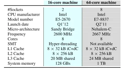
The analysis was carried out with several random lattices, gen-erated with Goldstein-Mayer bases, in multiple dimensions, avail-able on theSVP-challenge4 website. All lattices were generated with seed 0. Table 1 provides the specifications of the two test plat-forms, with 16 and 64 cores. The 16-core machine runs Ubuntu 11.10, kernel 3.0.0-32-generic, whereas the 64-core machine runs SUSE Linux Enterprise Server 11 SP3, kernel 3.0.101-0.29-default. The results were obtained on the 16-core machine, except in Sec-tion 5.2.3, where we present the scalability tests for both machines.
16-core machine 64-core machine
#Sockets 2 8
CPU manufacturer Intel Intel
Model number E5-2670 E7-8837
Launch date Q1’12 Q2’11
Micro-architecture Sandy Bridge Nehalem-C
Frequency 2600 MHz 2667 MHz
Cores 8 8
SMT Hyper-threading Not available
L1 Cache 8×32 kB iC+dC 8×32 kB iC+dC
L2 Cache 8×256 kB 8×256 kB
L3 Cache 20 MB shared 24 MB shared
System memory 128 GBs 1 TB
Table 1. Specifications of the test platforms. SMT stands for Si-multaneous multi-threading, iC/dC for instruction/data cache.
The code was compiled withIntel icpc 13.1.3, but the ex-periments in Section 5.2.1 include results forGNU g++ 4.6.1as well. We used the-O2optimization flag on both compilers, since it was slightly better than-O3. Every experiment was repeated three times and the best sample was chosen, although the runtimes usu-ally were quite stable among different runs. The elapsed time of lattice reduction is not included in the results. Target norms (cf. def-inition in Section 5.3.2) were never used, except in Section 5.3.2.
5.1 Performance comparison in sequential
In this section, we compare our parallel lock-free implementation of GaussSieve, from here on referred to asplfgsieve, running with a single thread, with (1) thefplll’s svpcall and (2) thegsieve li-brary, both overviewed in Section 3.1. The codes were compiled withicpcand the bases were BKZ-reduced. We used NTL’s im-plementation of BKZ5, with block-size 20. Althoughfplllhas it-self an implementation of BKZ, we stuck to NTL’s implementation of BKZ for all of the three SVP-solvers, since different implemen-tations of BKZ impact the performance of the solvers.
With higher block-sizes, BKZ finds the shortest vector per se, thus making comparisons of the solvers impossible: the execution time of the SVP-solvers would be nearly zero, since the elapsed time of the lattice reduction process is not included in the measure-ments.
We deactivated optimizationopt1 described in Section 4.4 in our implementation, because it renders the algorithm unstable for lattices in dimensions lower than 60, as also mentioned in Section 4.4. As for the stopping criterion, described in Section 2.3, we set α= 0.1andβ= 200, for bothgsieveandplfgsieve.
As Figure 1 shows, our version outperforms clearly thegsieve library, due to the use of vectorization andopt2. In particular, the difference of performance grows with the dimension of the lattice. For instance, our implementation is≈2.56x faster for a lattice in dimension 50, but≈4.45x and≈5.61x faster for lattices in dimen-sions 66 and 68. Moreover, the runtime of GaussSieve increases with the dimension of the lattice, regardless of the implementation.
4http://www.latticechallenge.org/svp-challenge/ 5http://www.shoup.net/ntl/
20 400 8000 160000
50 52 54 56 58 60 62 64 66 68 Lattice Dimension
fplll's svp gsieve plfgsieve
E
xe
cutio
n
Tim
e
(s)
Figure 1. Execution time, in seconds, forfplll’s svp,gsieveand plfgsieve(1 thread), on lattices in dimensions 50-68 (less is better).
The running time offplll’s svp, on the contrary, does not neces-sarily increase on a lattice in a higher dimension. For instance, the fplll’s svpis faster on the lattice in dimension 60 than on the lattice in dimension 58. Thefplll’s svpis slower than both implementa-tions of GaussSieve for lattices in higher dimensions than 54. In particular, the differences become very significant for high dimen-sions (e.g.≈40x slower thanplfgsievefor dimensions 64 and 66).
5.2 Performance of parallel lock-free GaussSieve
This section shows the assessment of the vectorization of the dot product kernel on our implementation, the impact of lattice reduc-tion on GaussSieve, and its scalability.
5.2.1 Vectorization and compiler’s impact
This section shows a quantitative performance evaluation of the vectorization of the kernel that computes the dot producthv,pi, the dominant kernel of the proposed implementation. The kernel was isolated and ran on synthetic vectors, in dimension 80, both 8- and 16-bytes aligned. In order to obtain solid numbers, the kernel was run 100 million times and the average performance was calculated. Table 2 presents the results of the benchmarks, when thedata
array, introduced in the beginning of Section 4.1, is 8-byte aligned. It includes the number of Cycles Per Element (CPE), where an el-ement is a multiplication ofvi andpi, in the dot producthv,pi.
The results differ considerably for different data-types and be-tween hand- and compiler-vectorized code. Both compilers per-form equally on code that is not hand-vectorized, forshort ar-rays, whereasg++ 4.6.1performs better thanicpc 13.1.3for not hand-vectorized code onintarrays, by a factor of≈1.39x. This picture changes for hand-vectorized code:icpc 13.1.3performs better thang++ 4.6.1for integer arrays, by a factor of≈2.74x, and a factor of≈2.70x is gained in operations onshortarrays.
For memory that is 16-byte aligned, the difference between the performance of both compilers is very similar to the results with 8-byte aligned memory. With integers, the performance of all scenarios and both compilers is actually, for two decimal places, the same as with memory that is 8-byte aligned. When it comes toshortarrays,icpc 13.1.3performs worse in code that is not hand-vectorized, but maintains the very same levels of performance in hand-vectorized code.gcc 4.6.1, on the other hand, performs worse in both hand and not hand-vectorized code. These results are shown in Table 3.
icpc 13.1.3 g++ 4.6.1
Time (s) CPEs Time (s) CPEs
Not hand-vectorized
integers 9.618 3.126 6.900 2.242
shorts 7.012 2.279 7.000 2.274
Hand-vectorized
integers 0.698 0.227 1.910 0.621
shorts 0.364 0.118 0.982 0.320
Table 2. Runtime, in seconds, and CPE of the dot product kernel, compiled with both icpc 13.1.3 and g++ 4.6.1. The time concerns 100 million runs of the kernel. Memory is 8-bytes aligned.
selected for benchmarks. On the basis of these results, the results in the remaining sections were obtained withicpc 13.1.3, except when said otherwise, and 8-byte aligned data.
icpc 13.1.3 g++ 4.6.1
Time (s) CPEs Time (s) CPEs Not hand-vectorized
integers 9.611223 3.123647 6.906026 2.244458
shorts 7.488067 2.433622 7.952487 2.584558
Hand-vectorized
integers 0.697577 0.226713 1.911845 0.621350
shorts 0.363973 0.118291 1.054764 0.342798
Table 3. Runtime, in seconds, and CPE of the dot product kernel, compiled with both icpc 13.1.3 and g++ 4.6.1. The time concerns 100 million runs of the kernel. Memory is 16-bytes aligned.
5.2.2 Impact of lattice reduction
While it is known that lattice reduction interferes with the perfor-mance of GaussSieve, the degree of this interference is not entirely known. In particular, different block-sizes in BKZ might greatly change the performance of GaussSieve. One of the reasons why the optimality of lattice reduction in this context is very hard to estimate, is because it depends not only on the dimension of the lattice but also from lattice to lattice. This means that different pa-rameters of BKZ might be optimal for a certain latticeLin a given dimensionn, but might be suboptimal for a different latticeQ, even ifQis in the same dimensionn.
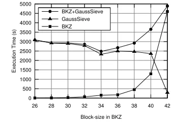
Although this subject deserves a thorough analysis by itself, we did conduct a small, yet useful, investigation on this mat-ter. This enables fair comparisons with other implementations of GaussSieve, such as those shown in Section 5.3. In particu-lar, we tested our implementation, running with 32 threads, on a 80-dimensional random lattice BKZ-reduced with different block-sizes, ranging from 26 to 42. The results are shown in Figure 2.
Considering the execution time of GaussSieve exclusively, the optimal block-size for the lattice reduction process, with BKZ, is 42. However, the execution time of BKZ increases with the block-size, and becomes a significant portion of the overall elapsed time for block-sizes bigger than 36. This means that even when GaussSieve is executed in a short time-frame, the combined execu-tion time might be substantially higher than in cases where BKZ is run with a small block-size. For instance, GaussSieve executes approximately 8 times faster when BKZ reduces the lattice with block-size 42 instead of 34. However, the combined elapsed time is almost 2 times smaller when BKZ runs with block-size 34. This
0 500 1000 1500 2000 2500 3000 3500 4000 4500 5000
26 28 30 32 34 36 38 40 42
Block-size in BKZ BKZ+GaussSieve GaussSieve BKZ
E
xe
cutio
n
Tim
e
(s)
Figure 2. Execution time, in seconds, of GaussSieve, BKZ and both combined for different block-sizes in BKZ.
is interesting because it seems a common practice to omit the ex-ecution time of the lattice reduction process, when reporting the execution times for SVP-solvers (e.g. [6, 12]).
The results in the following sections concern lattices that are BKZ-reduced with block-size 32 (except when said otherwise), because it is the most effective value from those in which the lattice reduction process represents<5% of the overall elapsed time.
5.2.3 Scalability
The scalability of our implementation on the 16-core machine was measured for random lattices in dimensions 60, 70 and 80. Lower dimensions are either solved very quickly or the lattice reduction process finds the shortest vector per se, rendering a scalability anal-ysis worthless. Running the implementation in higher dimensions, on the other hand, is impractical for a single thread.
We conducted two sets of experiments. In the first set, opt2, described in Section 4.4, was not activated. In the second set, on the contrary,opt2was activated. BKZ ran with block-size 20 for dimensions 60 and 70, and with block-size 32 for dimension 80. Running the implementation on lattices in dimensions 60 and 70 with the same block-size, of 32, is particularly fast, and no significant conclusions can be drawn about the results. Moreover, the parameter d, in dimension 60, was log(n)/30, because the default stopping criterion is insufficient ifdislog(n)/70instead. Thedataarray, which holds the coordinates of the vectors, was set to holdshorts in both sets of experiments.
scal-1 20 400 8000 160000
1 2 4 8 16 32
#Threads
Dim 80 Dim 70 Dim 60
E
xe
cutio
n
Tim
e
(s)
Figure 3. Scalability of our implementation on the 16-core ma-chine (with SMT) for 1-32 threads. Results for lattices in dimen-sions 60, 70 and 80. BKZ’s block-size is 32.opt1is turned off.
Dimension 60 Dimension 70 Dimension 80
Threads S E S E S E
First set of trials
2 2.00x 100% 1.96x 98.00% 1.92x 96%
4 3.88x 97.00% 4.09x 102.25% 3.82x 95.5%
8 7.35x 91.88% 8.06x 100.75% 7.35x 91.88%
16 13.36x 83.50% 15.36x 96.00% 13.58x 84.88%
32 17.18x 53.69% 20.25x 63.28% 21.20x 66.25%
Second set of trials
2 1.83x 91.85% 1.91x 95.50% 1.93x 96.50%
4 3.84x 96.00% 3.48x 87.00% 3.83x 95.75%
8 7.34x 91.75% 4.97x 62.13% 7.22x 90.25%
16 13.32x 83.25% 5.66x 35.38% 12.64x 79.00%
32 16.41x 51.29% 4.20x 13.13% 16.82x 52.56%
Table 4. Speedups (S) and Efficiency (E) of our implementation running on three random lattices (dimensions 60, 70 and 80). BKZ’s block-size set to 32. SMT is used in grayed out rows.
ability of this kernel is hurt by the use of, among others, a rand()-alike function. As this becomes the dominant kernel with this opti-mization, the scalability of the whole implementation is reduced. In fact, this is the only case where our implementation does not benefit from SMT. This problem is mitigated for higher dimensions, where the sampler is no longer the dominant kernel, as proven by the re-sults in dimension 80. It is unclear if higher dimensions might ben-efit from even more strict parameters in Klein’s algorithm, which
1 20 400 8000 160000
1 2 4 8 16 32
#Threads
Dim 80 Dim 70 Dim 60
E
xe
cutio
n
Tim
e
(s)
Figure 4. Scalability of our implementation on the 16-core ma-chine (with SMT) for 1-32 threads. Results for lattices in dimen-sions 60, 70 and 80. BKZ’s block-size is 32.opt1is turned on.
400 8000 160000
8 16 32 64
#Threads
Dim 78 Dim 76
E
xe
cutio
n
Tim
e
(s)
Figure 5. Scalability of our implementation on a 64-core machine, with 8-64 threads. Results for lattices in dimensions 76 and 78. BKZ’s block-size is 32.opt1is turned off.
might speedup GaussSieve but shift the computation weight to the Klein’s algorithm. Either way, we emphasize that (1) a more scal-able and efficient kernel of Klein’s algorithm must be developed and (2) the proposed implementation of the GaussSieve kernel can be seen as a highly efficient and scalable building block in future implementations.
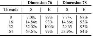
Figure 5 shows the execution times of our implementation on the 64-core machine, for 8, 16, 32 and 64 threads. This corresponds to the use of one, two, four and eight CPU-chips, respectively. As we are primarily interested in the scalability of our GaussSieve kernel,opt1was deactivated in these tests. The version oficpcon this machine is 14.0.2 and the code was also compiled with-O2. As the figure shows, our implementation scales almost linearly for up to 64 threads. The speedups and efficiency are shown in Table 5. Our implementation scales linearly for a lattice in dimension 76 and almost linearly for a lattice in dimension 78. The running times are considerably slower than in the 16-core machine due to the differences in the microarchitectures.
Dimension 76 Dimension 78
Threads S E S E
8 7.08x 89% 7.74x 97%
16 14.84x 93% 14.86x 93%
32 32.02x 100% 29.65 93%
64 63.64x 99% 53.96x 84%
Table 5. Speedup (S) and Efficiency (E) of our implementation on the 64-core machine. BKZ’s block-size is 32.opt1is turned off.
5.3 Comparison of parallel performance
This section compares the performance of our implementation with the parallel GaussSieve implementations described in [12] and [6], recapped in Section 3. For the sake of simplicity, we refer to these asMilde2011andIshiguro2013, respectively. The trials were conducted on the 16-core machine, described in Section 5.
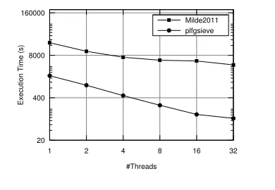
5.3.1 Comparison withMilde2011
We ran both implementations with 1-32 threads on a random lattice in dimension 70. Solving lattices in higher dimensions is imprac-tical for less than 32 threads. In this comparison, the lattice was BKZ-reduced, with block-size 32, and we deactivatedopt1in our implementation, since it degrades the scalability of the GaussRe-duce kernel, as mentioned in the previous section.
20 400 8000 160000
1 2 4 8 16 32
#Threads
Milde2011 plfgsieve
E
xe
cutio
n
Tim
e
(s)
Figure 6. Scalability of our implementation andMilde2011, for 1-32 threads on the 16-core machine (with SMT). Results for a lattice in dimension 70. BKZ’s block-size is 32.opt1is turned off.
than 10x, but it also scales much better. In particular, our implemen-tation achieves efficiency levels of 98%, 102.25%, 100.75%, 96% and 63.28% (the latter with SMT), whereasMilde2011 achieves only 92%, 69.56%, 42.75%, 22.62% and 14.92% (the latter with SMT) for 2, 4, 8, 16 and 32 threads, respectively.
5.3.2 Comparison withIshiguro2013
TheIshiguro2013implementation is not disclosed, and several im-plementation details, such as those discussed in Section 3.2, are omitted, thus making a re-implementation impossible. Neverthe-less, we can still compare our results with the execution times re-ported in the paper, since we use the same CPU-chip model. We also replicated the test environment: we ran our implementation with 32 threads, the execution time of the lattice pre-reduction (BKZ with block-size 30) was not measured.
Using 32 threads andr= 8.192, the authors reported an exe-cution time of 0.9 hours, i.e., 54 minutes or 3240 seconds, for the execution on a random lattice (seed 0) from theSVP-challenge, in dimension 80 (see Section 5.3, Table 2). The execution times for both a random and an ideal lattice are exactly the same, which is surprising, considering that substantial speedups (e.g.>50x) are possible to be achieved for GaussSieve on ideal lattices [14].
Despite of this, our implementation solves the very same lat-tice in 2896 seconds, i.e. less than 48 and a half minutes (or≈0.8 hours), which represents an improvement of nearly 12%. In fact, running theIshiguro2013implementation with an optimal value for rwould still require not less than 45 minutes, i.e. 2700 seconds (see Section 5.1, Figure 3(a)). This is equivalent to a more relaxed stop-ping criterion on our implementation, sincerdirectly influences the number of iterations required for convergence. In particular, one can compare this result to the most relaxed stopping criterion on our implementation, which is to set a target normtnas in [15], that permits the algorithm to stop as soon as a vector with norm smaller or equal totnis found. In this case, with the same 32 threads and BKZ’s block-size 30, our implementation runs in 1788 seconds, which represents an improvement factor of more than 1.5x.
The authors do not present or comment on the impact of BKZ’s block-size on the performance of the GaussSieve, and therefore we assume that 30 is the optimal choice for this parameter on their implementation. On the contrary, we did assess the impact that different block-sizes in BKZ have on the performance of our implementation, as shown in Section 5.2.2. In particular, for BKZ with block-size 34, our implementation solves the SVP on the aforementioned lattice in≈2328 and≈1591 seconds, respectively with and without a target norm set. These numbers mean that our implementation is faster by a factor between≈1.39x and≈1.7x.
6.
Conclusions and Outlook
This paper proposes a parallel implementation of GaussSieve, an important heuristic that solves the SVP. We show that, by slightly relaxing the properties of GaussSieve, it is possible to achieve almost linear and linear speedups up to 64 cores, depending on the tested scenario. The core idea of the proposed implementation is a lock-free list that holds the vectors in the system, combined with hand-vectorized and hand-optimized code.
In comparison to the previously proposed parallel implementa-tions of GaussSieve, our implementation performs and scales much better thanMilde2011, and outperformsIshiguro2013, by factors of between nearly 1.12x and 1.50x, for lattices that are BKZ-reduced with block-size 32, and between nearly 1.39x and 1.70x, for lattices that are BKZ-reduced with block-size 34.
In the future, we plan to adapt our algorithm to work on ideal lattices, and implement it on CPU+GPU frameworks (e.g. [9]). In this version, we plan to integrate the improvements proposed in [3]. We also plan to implement a parallel version of BKZ on GPUs.
Acknowledgements
We thank M. Schneider for providing us the implementation showed in [12], and ¨O. Dagdelen, L. Santos, T. Laarhoven and F. Correia for insightful discussions. This work was partially sup-ported by the German Science Foundation through SFB 1119 (CROSSING).
References
[1] M. Ajtai. The Shortest Vector Problem in L2 is NP-hard for Random-ized Reductions (Extended Abstract). InProceedings of the Thirtieth Annual ACM Symposium on Theory of Computing, STOC ’98, pages 10–19, New York, NY, USA, 1998. ACM.
[2] M. Ajtai et al.. A Sieve Algorithm for the Shortest Lattice Vector Problem. InProceedings of the Thirty-third Annual ACM Symposium on Theory of Computing, STOC ’01, pages 601–610, New York, NY, USA, 2001. ACM.
[3] R. Fitzpatrick et al. Tuning GaussSieve for Speed. InThird Inter-national Conference on Cryptology and Information Security in Latin America (Latincrypt), Florianopolis, Brazil, September 2014. [4] N. Gama, P. Nguyen, and O. Regev. Lattice Enumeration Using
Ex-treme Pruning. In H. Gilbert, editor,Advances in Cryptology - EU-ROCRYPT 2010, volume 6110 ofLecture Notes in Computer Science, pages 257–278. Springer Berlin Heidelberg, 2010.
[5] T. L. Harris. A Pragmatic Implementation of Non-blocking Linked-Lists. InProceedings of the 15th International Conference on Dis-tributed Computing, DISC ’01, pages 300–314, London, UK, UK, 2001. Springer-Verlag.
[6] T. Ishiguro et al.. Parallel Gauss Sieve Algorithm : Solving the SVP in the Ideal Lattice of 128-dimensions. Cryptology ePrint Archive, Report 2013/388, 2013.
[7] P. Klein. Finding the Closest Lattice Vector when It’s Unusually Close. InProceedings of the Eleventh Annual ACM-SIAM Symposium on Discrete Algorithms, SODA ’00, pages 937–941, Philadelphia, PA, USA, 2000. Society for Industrial and Applied Mathematics. [8] T. Laarhoven et al.. Solving Hard Lattice Problems and the Security
of Lattice-Based Cryptosystems. Cryptology ePrint Archive, Report 2012/533, 2012.
[9] A. Mariano et al.. A (ir)regularity-aware task scheduler for hetero-geneous platforms. InProceedings of the Second International Con-ference on High Performance Computing, HPC-UA’12, pages 45–56, Kiev, Ukraine, October, 8-10 2012.
[11] D. Micciancio and P. Voulgaris. Faster exponential time algorithms for the shortest vector problem. InProceedings of the Twenty-First Annual ACM-SIAM Symposium on Discrete Algorithms, SODA ’10, pages 1468–1480, Philadelphia, PA, USA, 2010. SIAM2.
[12] B. Milde and M. Schneider. A parallel implementation of GaussSieve for the shortest vector problem in lattices. InProceedings of the 11th International Conference on Parallel computing technologies, PaCT’11, pages 452–458, Berlin, Heidelberg, 2011. Springer-Verlag. [13] P. Q. Nguyen and et al. Sieve algorithms for the shortest vector
problem are practical.J. of Mathematical Cryptology, 2(2), 2008. [14] M. Schneider. Analysis of Gauss-Sieve for Solving the Shortest Vector
Problem in Lattices. InWALCOM: Algorithms and Computation, volume 6552 ofLecture Notes in Computer Science, pages 89–97. Springer Berlin Heidelberg, 2011.
[15] M. Schneider. Sieving for Shortest Vectors in Ideal Lattices. In
Progress in Cryptology AFRICACRYPT 2013, volume 7918 of Lec-ture Notes in Computer Science, pages 375–391. Springer Berlin Hei-delberg, 2013.
[16] P. Xavier et al.. Solving the shortest lattice vector problem in time 22.465n. Cryptology ePrint Archive, Report 2009/605, 2009. [17] W. Xiaoyun et al.. Improved Nguyen-Vidick heuristic sieve algorithm
for shortest vector problem. InIn Proceedings of ASIACCS 11, pages 1–9. ACM, 2011.