On the Complexity of the BKW Algorithm on LWE
Martin R. Albrecht1, Carlos Cid3, Jean-Charles Faug`ere2, Robert Fitzpatrick3, and Ludovic Perret2 1 Technical University of Denmark, Denmark
2
INRIA, Paris-Rocquencourt Center, POLSYS Project UPMC Univ Paris 06, UMR 7606, LIP6, F-75005, Paris, France
CNRS, UMR 7606, LIP6, F-75005, Paris, France 3
Information Security Group Royal Holloway, University of London Egham, Surrey TW20 0EX, United Kingdom
[email protected], [email protected], [email protected], [email protected], [email protected]
Abstract. This work presents a study of the complexity of the Blum-Kalai-Wasserman (BKW) algo-rithm when applied to the Learning with Errors (LWE) problem, by providing refined estimates for the data and computational effort requirements for solving concrete instances of the LWE problem. We apply this refined analysis to suggested parameters for various LWE-based cryptographic schemes from the literature and compare with alternative approaches based on lattice reduction. As a result, we provide new upper bounds for the concrete hardness of these LWE-based schemes. Rather surprisingly, it appears that BKW algorithm outperforms known estimates for lattice reduction algorithms starting in dimensionn ≈250 when LWE is reduced to SIS. However, this assumes access to an unbounded number of LWE samples.
1
Introduction
LWE (Learning with Errors) is a generalisation for large moduli of the well-known LPN (Learning Parity with Noise) problem. It was introduced by Regev in [29] and has provided cryptographers with a remarkably flexible tool for building cryptosystems. For example, Gentry, Peikert and Vaikuntanathan presented in [17] LWE-based constructions of trapdoor functions and identity-based encryption. Moreover, in his recent semi-nal work Gentry [16] resolved one of the longest standing open problems in cryptography with a construction related to LWE: the first fully homomorphic encryption scheme. This was followed by further constructions of (fully) homomorphic encryption schemes based on the LWE problem, e.g. [5, 11]. Reasons for the popu-larity of LWE as a cryptographic primitive include its simplicity as well as convincing theoretical arguments regarding its hardness, namely, a reduction from worst-case lattice problems, such as the (decision) Shortest Vector Problem (GapSVP) and Short Independent Vectors Problem (SIVP), to average-case LWE [29, 10].
Definition 1 (LWE [29]).Letn, qbe positive integers,χbe a probability distribution onZandsbe a secret vector following the uniform distribution on Zn
q. We denote byLs,χ the probability distribution on Znq ×Zq
obtained by choosinga from the uniform distribution on Zn
q, choosing e∈Z according to χ, and returning (a, c) = (a,ha,si+e)∈Znq ×Zq.
–Search-LWEis the problem of findings∈Znq given pairs (ai, ci)∈Znq ×Zq sampled according to Ls,χ.
–Decision-LWEis the problem of deciding whether pairs(ai, ci)∈Znq×Zq are sampled according to Ls,χ or
The modulus q is typically taken to be polynomial inn, and χ is the discrete Gaussian distribution on Z with mean 0 and standard deviationσ=α·q, for someα.1For these choices it was shown in [29, 10] that if
√
2πσ >2√n, then (worst-case) GapSVP−O˜(n/α) reduces to (average-case) LWE.
Motivation. While there is a reduction of LWE to (assumed) hard lattice problems [29], little is known about theconcretehardness of particular LWE instances. That is, given particular values forσ,qandn, what is the computational cost to recover the secret using currently known algorithms? As a consequence of this gap, most proposals based on LWE do not provide concrete choices for parameters and restrict themselves to asymptotic statements about security, which can be considered unsatisfactorily vague for practical purposes. In fact we see this lack of precision as one of the several obstacles to the consideration of LWE-based schemes for real-world applications.
Previous Work.We may classify algorithms for solving LWE into two families. The first family reduces LWE to the problem of finding a short vector in the (scaled) dual lattice (commonly known as the Short In-teger Solution (SIS) problem) constructed from a set of LWE samples. The second family solves the Bounded Distance Decoding (BDD) problem in the primal lattice. For both families lattice reduction algorithms may be applied. We may either use lattice reduction to find a short vector in the dual lattice or apply lattice reduction and (a variant of) Babai’s algorithm to solve BDD [21]. Indeed, the expected complexity of lattice algorithms is often exclusively considered when parameters for LWE-based schemes are discussed. However, while the effort on improving lattices algorithms is intense [31, 12, 26, 15, 27, 19, 25, 28], our understanding of the behaviour of these algorithms in high dimensions is still limited.
On the other hand, combinatorial algorithms for tackling the LWE problem remain rarely investigated from an algorithmic point of view. For example, the main subject of this paper – the BKW algorithm – specifically applied to the LWE problem has so far received no treatment in the literature2. However, since the BKW algorithm can be viewed as an oracle producing short vectors in the dual lattice spanned by theai (i.e., it reduces LWE to SIS) it shares some similarities with combinatorial (exact) SVP solvers. Finally, recently a new algorithm for LWE that reduces the problem to BDD but does not make calls to lattice reduction algorithms has been proposed: Arora and Ge [7] proposed a new algebraic technique for solving LWE. The algorithm has a total complexity (time and space) of 2O˜(σ2) and is thus subexponential when σ ≤ √n, remaining exponential when σ > √n. It is worth noting that Arora and Ge achieve the √n hardness-threshold found by Regev [29], and thus provide a subexponential algorithm precisely in the region where the reduction to GapSVP fails. We note however that currently the main relevance of Arora-Ge’s algorithm is asymptotic as the constants hidden in ˜O(·) are rather large [3]; it is an open question whether one can improve its practical efficiency.
Contribution.Firstly, we present a detailed study of a dedicated version of the Blum, Kalai and Wasserman (BKW) algorithm [9] for LWE with discrete Gaussian noise. The BKW algorithm is known to have (time and space) complexity 2O(n)when applied to LWE instances with a prime modulus polynomial inn[29]; in this paper we provide both the leading constant of the exponent in 2O(n) and concrete costs of BKW when applied to Search- and Decision-LWE. That is, by studying in detail all steps of the BKW algorithm, we ‘de-asymptotic-ify’ the understanding of the hardness of LWE under the BKW algorithm and provide concrete values for the expected number of operations for solving instances of the LWE problem. More precisely, we show the following theorem in Section 3.4.
1
It is common in the literature on LWE to parameterise discrete Gaussian distributions bys=σ√2πinstead ofσ. Since we are mainly interested in the “size” of the noise, we deviate from this standard in this work.
2
Theorem 1 (Search-LWE, simplified). Let (ai, ci) be samples following Ls,χ, set a=blog2(1/(2α)2)e, b = n/a and q a prime. Let d be a small constant 0 < d < log2(n). Assume α is such that qb =qn/a = qn/blog2(1/(2α)2)e
is superpolynomial in n. Then, given these parameters, the cost of the BKW algorithm to solve Search-LWEis
qb−1 2
·
a(a
−1)
2 ·(n+ 1)
+
qb 2
·ln
d
m
+ 1·d·a+ poly(n)≈ a2n·q
b
2
operations inZq. Furthermore,
a·
qb 2
+ poly(n)calls toLs,χ and storage of
a·
qb 2
·n
elements inZq are needed.
We note that the above result is a corollary to our main theorem (Theorem 2) which depends on a value m. However, since at present no closed form expressingm is known, the above simplified statement avoids mby restricting choices on parameters of the algorithm. We also show the following simple corollary on the algorithmic hardness of Decision-LWE.
Corollary 1 (Decision-LWE).Let (ai, ci)be samples followingLs,χ,0< b≤nbe a parameter,0< <1
the targeted success rate and a=dn/be the addition depth. Then, the expected cost of the BKW algorithm to distinguish Ls,χ from random with success probability is
qb−1 2
·
a(a−1)
2 ·(n+ 1)−
ba(a−1)
4 −
b 6
(a−1)3+3 2(a−1)
2+1 2(a−1)
additions/subtractions inZq to produce elimination tables,
m·a
2 ·(n+ 2)
withm=/exp
−π
2σ22a+1 q2
additions/subtractions in Zq to produce samples. Furthermore, a·lq2bm+m calls to Ls,χ and storage for
qb
2
·a· n+ 1−ba−21elements in Zq are needed.
This corollary is perhaps the more useful result for cryptographic applications which rely on Decision-LWE and do not assume a prime modulus q. Here, we investigate the search variant first because the decision variant follows easily. However, we emphasize that there are noticeable differences in the computational costs of the two variants. A reader only interested in Decision-LWE is invited to skip Sections 3.2 and 3.3.
2
Preliminaries
Gaussians.LetN(µ, σ2) denote the Gaussian distribution with meanµand standard deviationσ. The LWE problem considers a discrete Gaussian distribution overZwhich is then reduced moduloq. This distribution in Zq can be obtained by discretising the corresponding wrapped Gaussian distribution over the reals. To wrapN(0, σ2) modq, we denote byp(φ) the probability density function determined byσ, define the periodic variableθ:=φmodq and let
p0(θ) =
∞
X
k=−∞
p(θ+qk) for −q/2< θ≤q/2. (1)
As |k| increases, the contribution of p(θ+qk) falls rapidly; in fact, exponentially fast [13]. Hence, we can pick a point at which we ‘cut’p0(θ) and work with this approximation. We denote the distribution sampled according top0 and rounded to the nearest integer in the interval ]−2q,2q] byχα,q, whereσ=α·q. That is,
Pr[X=x] =
Z x+12
x−1 2
p0(t)dt (2)
We note that, in our cases of interest, we can explicitly compute Pr[X=x] because bothqandkare poly(n).
We state a straightforward lemma which will be useful in our computations later.
Lemma 1. Let X0, . . . , Xm−1 be independent random variables, withXi ∼ N(µ, σ2). Then their sum X =
Pm−1
i=0 Xi is also normally distributed, withX∼ N(mµ, mσ 2).
In the case ofXifollowing a discrete Gaussian distribution, it does not necessarily follow that a sum of such random variables is distributed in a way analogous to the statement above. However, throughout this work, we assume that this does hold i.e., that Lemma 1 applies to the discrete Gaussian case - while we do not know how to prove this, this assumption causes no apparent discrepancies in our experimental results. For a detailed discussion on sums of discrete Gaussian random variables, the interested reader is referred to [1].
Computational Model.We express concrete costs as computational costs and storage requirements. We measure the former inZq operations and the latter in the number ofZqelements requiring storage. However, as the hardness of LWE is related to the quantity nlogq [10], relying on these measures would render results for different instances incommensurable. We hence normalise these magnitudes by considering “bit-operations” where one ring operation inZq is equivalent to log2qsuch bit operations. The specific multiplier log2qis derived from the fact that the majority of operations are additions and subtractions inZq as opposed to multiplications in Zq. In particular, we ignore the cost of “book keeping” and of fixed-precision floating point operations occuring during the algorithm (where the precision is typically a small multiple of n, cf. Section 4).
still hold. Similar notions (in the case of LPN) were considered in [14], although, as in this work, the authors did not analyse the impact of these steps.
Notation.We always start counting at zero, and denote vectors in bold. Given a vectora, we denote bya(i) thei-th entry ina, i.e., a scalar, and bya(i,j)the subvector of aspanning the entries at indicesi, . . . , j−1. When given a list of vectors, we index its elements by subscript, e.g., a0,a1,a2, to denote the first three vectors of the list. When we write (ai, ci) we always mean the output of an oracle which should be clear from the context. In particular, (ai, ci) does not necessarily refer to samples following the distributionLs,χ.
3
The BKW Algorithm
The BKW algorithm was proposed by Blum, Kalai and Wasserman [9] as a method for solving the LPN problem, with sub-exponential complexity, requiring 2O(n/logn) samples and time. The algorithm can be adapted for tackling Search- and Decision-LWE, with complexity 2O(n), when the modulus is taken to be polynomial inn.
To describe and analyse the BKW algorithm we use terminology and intuitions from linear algebra. Recall that noise-free linear systems of equations are solved by (a) transforming them into a triangular shape, (b) recovering a candidate solution in one variable for the univariate linear equation produced and (c) extending this solution by back substitution. Similarly, if we are only interested indeciding whether a linear system of equations does have a common solution, the standard technique is to produce a triangular basis and express other rows as linear combinations of this basis, i.e., to attempt to reduce them to zero.
The BKW algorithm – when applied to Search-LWE – can be viewed as consisting of three stages somewhat analogous to those of linear system solving:
(a) sample reduction is a form of Gaussian elimination which, instead of treating each component inde-pendently, considers ‘blocks’ ofb components per iteration, whereb is a parameter of the algorithm.
(b) hypothesis testing tests candidate sub-solutions to recover components of the secret vectors.
(c) back substitution such that the whole process can be continued on a smaller LWE instance.
On a high-level, to aid intuition, if the standard deviation ofχwas zero and hence all equations were noise-free, we could obviously recover sby simple Gaussian elimination. When we have non-zero noise, however, the number of row-additions conducted during Gaussian elimination result in the noise being ‘amplified’ to such levels that recovery ofswould generally be impossible. Thus the motivation behind the BKW algorithm can be thought of as using a greater number of rows but eliminating many variables with single additions of rows rather than just one. If we can perform a Gaussian elimination-like reduction of the sample matrix using few enough row additions, the resulting noise in the system is still ‘low enough’ to allow us to recover one or a few components ofsat a time. While, mainly for convenience of analysis, we choose a nested-oracle approach below to define the algorithm, the above intuitive approach is essentially equivalent.
The way we study the complexity of the BKW algorithm for solving the LWE problem is closely related to the method described in [14]: given an oracle that returns samples according to the probability distributionLs,χ, we use the algorithm’s first stage to construct an oracle returning samples according to another distribution, which we call Bs,χ,a, where a = dn/bedenotes the number of ‘levels’ of addition. The complexity of the algorithm is related to the number of operations performed in this transformation, to obtain the required number of samples for hypothesis testing.
3.1 Sample Reduction
Given n∈Z, select a positive integer b≤n (the window width), and leta:=dn/be(the addition depth). Given an LWE oracle (which by abuse of notation, we will also denote by Ls,χ), we denote by Bs,χ,` a related oracle which outputs samples where the first b·` coordinates of each ai are zero, generated under the distribution (which again by abuse of notation, we denote byBs,χ,`) obtained as follows:
– if`= 0, then Bs,χ,0 is simplyLs,χ;
– if 0< ` < a, the distributionBs,χ,`is obtained by taking the difference of two vectors fromBs,χ,`−1 that agree on the elements (a((`−1)·b),a((`−1)·b+1), . . . ,a(`·b−1)).
We can then describe the first stage of the BKW algorithm as the (recursively constructed) series of sample oraclesBs,χ,`, for 0≤` < a. Indeed, we defineBs,χ,0 as the oracle which simply returns samples fromLs,χ, whileBs,χ,`is constructed fromBs,χ,`−1, for`≥1. We will make use of a set of tablesT (maintained across oracle calls) to store (randomly-chosen) vectors that will be used to reduce samples arising from our oracles. More explicitly, given a parameterb≤nfor the window width, and lettinga=dn/be, we can describe the oracleBs,χ,`as follows:
1. For `= 0, we can obtain samples from Bs,χ,0 by simply calling the LWE oracleLs,χ and returning the output.
2. For`= 1, we repeatedly query the oracleBs,χ,0to obtain (at most) (qb−1)/2 samples (a, c) with distinct non-zero vectors for the firstbcoordinates ofa. We only collect (qb−1)/2 such vectors because we exploit the symmetry of Zq and that of the noise distribution. We use these samples to populate the tableT1, indexed by the first b entries of a. We store (a, c) in the table. During this course of this population, whenever we obtain a sample (a0, c0) from Bs,χ,0, if either the firstb entries of a0 (resp. their negation) match the firstbentries of a vectorasuch that the pair (a, c) is already inT1, we return (a0±a, c0±c),
as a sample fromBs,χ,1. Note that, if the firstbentries ina0 are zero, we return (a0, c0) as a sample from Bs,χ,1. Further calls to the oracleBs,χ,1 proceed in a similar manner, but using (and potentially adding entries to) the same tableT1.
3. For 1 < ` < a, we proceed as above: we make use of the table T` (constructed by calling B
s,χ,`−1 up to (qb−1)/2 times) to reduce any output sample fromB
s,χ,`−1 which has thebentries in its`-th block already in T`, to generate a sample fromB
s,χ,`.
Input:b – an integer 0< b≤n
Input:` – an integer 0< ` < a
begin
T`←array indexed by
Zbq maintained across all runs ofBs,χ,`; queryBs,χ,`−1to obtain (a, c);
if a(b·(`−1),b·`) is all zero vector then
return(a, c);
while T`
a(b·(`−1),b·`)=∅and T
`
−a(b·(`−1),b·`)=∅do
T`
a(b·(`−1),b·`)←(a, c);
queryBs,χ,`−1to obtain (a, c);
if a(b·(`−1),b·`) is all zero vector then
return(a, c);
if T`
a(b·(`−1),b·`)6=∅then
(a0, c0)←Ta`(b·(`−1),b·`);
return(a−a0, c−c0);
else
(a0, c0)←T−`a
(b·(`−1),b·`);
return(a+a0, c+c0);
Algorithm 1:Bs,χ,`for 0< ` < a
Then, given an LWE oracleLs,χ outputting samples of the form (a,ha,si+e), wherea,s∈Znq, the oracle Bs,χ,a−1can be seen as another LWE oracle outputting samples of the form (a0,ha0,s0i+e0), wherea0,s0∈Zkq, withk=nmodb, ifbdoes not dividen, ork=botherwise, ande0is generated with a different distribution (related to the original error distribution and the valuea). The vectors0is defined to be the lastkcomponents of s. For the remainder of this section we will assume that nmodb = 0, and therefore k=b (this is done to simplify the notation, but all the results obtained can be easily adapted when the last block has length k < b).
We note that, in our analysis below, we make the assumption for simplicity that all tables are completely filled during the elimination stage of the algorithm, thus giving conservative time and space bounds. In practise, especially in the final tables, this will not be the case and birthday-paradox arguments could be applied to derive a more realistic (lower) complexity. Typically, if the number of samples required for hypothesis-testing is small, the birthday paradox implies that the storage required for the final table can be reduced by a square-root factor.
Moreover, in this work we introduce an additional parameter d ≤ b which does not exist in the original BKW algorithm [9]. This parameter is used to reduce the number of hypotheses that need to be tested in the second stage of the algorithm, and arises from the fact we work with primes q > 2. At times, instead of working with the last block of lengthb, which could lead to potentially exponentially many hypotheses qb to be tested, we may employ a final reduction phase –Bs,χ,a – to reduce the samples to d < bnon-zero entries ina. Thusdwill represent the number of components in our final block, i.e., the number of elements of the secret over which we conduct hypothesis tests. So after running theBs,χ,a−1algorithm, we may decide to split the final block to obtain vectors overZdq. If so, we run the reduction function described above once more, which we will denote byBs,χ,a. In the simple case where we do not split the last block (i.e.,d=b), we adopt the convention that we will also call theBs,χ,a function, but it will perform no extra action (i.e., it simply callsBs,χ,a−1). Thus we have that for a choice of 0≤d≤b, the oracleBs,χ,a will output samples of the form (a0,ha0,s0i+e0), wherea0,s0 ∈Zd
On choosing b andd.In general, as discussed above, choosing the parameter dto be small (e.g. 1 or 2) leads to the best results. However, in general one could also relax the conditiond≤bto d≤nwhered=n is equivalent to straight-forward exhaustive search. Finally, a natural question is – should all the blocks be of equal length or should some be shorter than others? Intuitively, choosing blocks which are all of equal size (or as close as possible) appears to be the optimal strategy, though we do not formally investigate this here. To ease the presentation, we assume throughout this paper that this is the case.
From the constructions above, it follows that the cost of one call toBs,χ,`is at mostdqb/2ecalls toBs,χ,`−1. We also need at most one addition of two outputs ofBs,χ,`−1, which have the firstb·`entries in common. This operation requiresn+ 1−b·`additions inZq. Furthermore, since we maintainT`across different runs ofBs,χ,`, this cost is amortised across different runs ofBs,χ,`. Hence, when` >0 the cost of callingBs,χ,` a total ofmtimes is upper bounded by:
m+q b−1
2 calls toBs,χ,`−1 andmadditions of outputs ofBs,χ,`−1. Overall we obtain Lemma 2.
Lemma 2. Let n≥1 be the dimension of the LWE secret vector, q be a positive integer, andd, b∈Z with
1≤d≤b≤n, and define a=dn/be. The cost of callingBs,χ,a, which returns samples(ai, ci) with at most
the drightmost entries of ai non-zero,m times is upper bounded by
qb−1 2
·
a(a
−1)
2 ·(n+ 1)−
ba(a−1)
4 −
b 6
(a−1)3+3 2(a−1)
2+1 2(a−1)
+m·a
2 ·(n+ 2)
<
qb−1 2
·
a(a−1)
2 ·(n+ 1)
+m·(a
2 ·(n+ 2))
additions inZq anda·
lqb
2
m
+m calls toLs,χ.
Proof. We may think of theBs,χ,`oracles as constructing the matrix
B = T1
0 . . .0T2
0 . . .0 0 . . .0T3 ..
. . .. ... ... . .. ... ... . .. 0 . . .0 0 . . .0 0 . . .0Ta−1 0 . . .0 0 . . .0 0 . . .0 0 Ta
0 . . .0 0 . . .0 0 . . .0 . . . 0 M
where, for 1≤i≤a−1,Ti represents a submatrix of (qb−1)/2 rows andn+ 1−b·(i−1) columns (the +1 accounts for theci column). According to our convention,Ta is either a submatrix of (qb−d−1)/2 rows and n+ 1−b·(a−1) columns if we split the last block (i.e.d < b), or an empty matrix. FinallyM represents a submatrix withm rows and d+ 1 columns. The matrix B has therefore at most (a−1)·((qb−1)/2) + ((qb−d−1)/2) +m < a·lqb
2
m
+mrows and hence needs as many calls toLs,χto be constructed. This proves the second claim.
For the upper-bound on the number of additions necessary inZq, we have the following (we treat the worst case, where full construction of all T tables is necessary before obtaining any samples from Bs,χ,a): The construction ofa T-tables is required, onlya−1 (at most) of which require additions.
2. The construction of tableT2 requires at most ((qb−1)/2)·(n+ 1−b) additions.
3. The construction of tableT3 requires at most ((qb−1)/2)·((n+ 1−b) + (n+ 1−2b)) additions. 4. In general, for 2< i < a, the construction of tableTi requires at most
qb−1 2
·
(i−1)·(n+ 1)−
i−1
X
j=1 j·b
=
qb−1 2
·(i−1)·
(n+ 1)− i
2 ·b
.
5. The construction of Ta - the above expression is an upper bound fori=a. 6. Thus, the construction of all theTi tables requires at most
qb−1 2 · a X j=2
(j−1)·((n+ 1)−j
2 ·b)
=
qb−1 2
· a(a−1)
2 ·(n+ 1)− a−1
X
k=1
k(k+ 1) 2 ·b
!
=
qb−1 2
·
a(a−1)
2 ·(n+ 1)−
ba(a−1)
4 −
b 6
(a−1)3+3 2(a−1)
2+1 2(a−1)
additions in Zq.
7. Now, for the construction of our mfinal samples, the construction of each of these samples requires at most
(n+ 1−b) + (n+ 1−2b) +. . .+ (n+ 1−a·b) = a
X
i=1
(n+ 1−ib)
< a·(n+ 1)−n
2
=a
2 ·(n+ 2)
additions (inZq).
8. Thus, the number of additions (in Zq) incurred through callingBs,χ,amtimes is upper-bounded by:
qb−1 2
·
a(a−1)
2 ·(n+ 1)−
ba(a−1)
4 −
b 6
(a−1)3+3 2(a−1)
2+1 2(a−1)
+m·a
2 ·(n+ 2)
and this concludes the proof of the lemma. ut
The memory requirements for storing the tablesTi are established in Lemma 3 below.
Lemma 3. Letn≥1be the dimension of the secret,qbe a positive integer, andd, b∈Zwith1≤d≤b≤n, and define a=dn/be. The memory required to store the tableTi is upper bounded by
qb 2
·a·
n+ 1−ba−1 2
Zq elements, each of which requiresdlog2(q)ebits of storage.
Proof. The table T1 has q2b entries each of which holds n+ 1 elements of Zq. The table T2 has the same number of entries but holds onn+ 1−belements ofZq. Overall, we get that all tables together hold
a X i=1 qb 2 ·
n+ 1−(i−1)b
= qb 2 a X i=1
n+ 1−(i−1)b
=
qb 2
·a·
n+ 1−ba−1 2
Note however that, while the original LWE oracleLs,χ may output zero vectors (which offer no information for the hypothesis tests in the search variant) with probability q−n, the oracle Bs,χ,a may output such zero vectors with noticeable probability. In particular, callingBs,χ,a mtimes does not guarantee that we get m samples with non-zero coefficients in ai. The probability of obtaining a zero vector from Bs,χ,a is q1d, and
thus expect to have to call the oracleBs,χ,a aroundqd/(qd−1)·mtimes to obtain≈museful samples with good probability.
3.2 Hypothesis Testing
To give concrete estimates for the time and data complexity of solving a Search-LWE instance using BKW, we formulate the problem of solving an LWE instance as the problem of distinguishing between two different distributions. Assume we have m samples in Zd
q ×Zq from Bs,χ,a. It follows that we have Zdq hypotheses to test. In what follows, we examine each hypothesis in turn and derive a hypothesised set of noise values as a result (each one corresponding to one of the msamples). We show that if we have guessed incorrectly for the subvectors0 ofsthen the distribution of these hypothesised noise elements will be (almost) uniform while if we guess correctly then these hypothesised noise elements will be distributed according toχa. That is, if we have that the noise distribution associated with samples fromLs,χisχ=χα,q, then it follows from Lemmas 1 and 2 that the noise distribution of samples obtained from Bs,χ,` follows χ√2`α,q if all inputs
are independent, i.e., we are adding 2` discrete Gaussians and produce a discrete Gaussian with standard deviation increased by a factor of √2`. For the sake of simplicity, we denote this distribution by χ` in the remainder of this work and also assume that the oracleBs,χ,a performs non-trivial operations on the output of Bs,χ,a−1, i.e., the oracle Bs,χ,a performs a further reduction step. In other words we assume that the final oracleBs,χ,a results in a further increase in the standard deviation of the noise distribution associated with the final samples which are used to test hypotheses for elements of s. We hence make the following assumption in this section:
Assumption 1 If we let s0:=s(n−d,n)= (s(n−d), . . . ,s(n−1)), then the output ofBs,χ,a is generated as
a←$Zdq, e←$χa : (a,ha,s0i+e).
Remark 1. This section only refers to the Search-LWE problem in which we assumeq is prime for ease of analysis and exposition. This restriction does not apply to our results below on the decision variant.
For our hypothesis-testing strategies, we think of each of the samples returned by Bs,χ,a as giving rise to many equations
fi=−ci±j+ d−1
X
k=0
(ai)(k)x(k)for 0≤j < q/2.
Given a number of these samples, in order to get an estimate for s0, we run through qd hypotheses and compute an array of scoresS indexed by the possible guesses inZd
q. That is, a functionW assigns a weight to elements in Zq which represent the noise under the hypothesis s0 = v. For each guess v we sum over the weighted noisesW(−ci+Pd−1
Input:F – a set ofmsamples followingBs,χ,a
Input:W – a weight function mapping members ofZq to real numbers
begin
S ←array filled with zeros indexed byZd q;
for v∈Zd q do wv← ∅;
forfi∈F do
write fi as−ci+Pd−1
k=0(ai)(k)·x(k); j ← hai,vi −ci;
wv←wv∪ {W(j)}; Sv←Pwi∈wvwi/m;
returnS
Algorithm 2: Analysing candidates.
Lemma 4. Running hypothesis testing costsm·qd operations in Zq.
Proof. Evaluatinghai,vi −ci at some point inZdq naively costs 2doperations inZq which implies an overall cost of 2d·m·qd. However, we can reorder the elements in
Zdq such that the element at indexhdiffers from the element at index h+ 1 by an addition of a unit vector inZd
q. Evaluating hai,vi −ci on all Zdq points ordered in such a way reduces to one operation in Zq: addition of ai,(j) wherej is the index at which two consecutive elements differ. Hence, Algorithm 2 costsm·qdoperations in Zq. ut
Recall that χa is the distribution of the errors under a right guess. Now, letUa denote the distribution of errors under a wrong guess v 6= s0. By the Neyman-Pearson Lemma, the most powerful test of whether samples follow one of two known distributions is the log-likelihood ratio.
Hence, forj, with d−q/2e ≤j≤ bq/2c, we set:
W(j) := log2
Pr[e←
$χa:e=j] Pr[e←$Ua:e=j]
. (3)
Next, we establish the relation between ˜pj := Pr[e←$Ua:e=j] and pj := Pr[e←$χa:e=j].
Lemma 5. Given a wrong guess v for s0, for each element fi = −ci +Pd−1
k=0(ai)(k)x(k) ∈ Zq[x], with ci =hai,s0i −ei, the probability of errorj appearing is
˜
pj:= Pr[e←$Ua:e=j] =
qd−1−p j
qd−1 (4)
if qis prime.
Proof. We writev=s0+t. Sincev is a wrong guess, we must havet=6 0. For a fixeds0 and for ai,t6=0, it holds that:
˜
pj= Pr[e←$Ua:e=j] = Pr[hai,vi −ci=j] = Pr[hai,ti −ei=j]
=
bq/2c
X
y=d−q/2e
Pr[ d−1
X
k=0
ai(k)t(k)=y]·Pr[j+ei=y]
!
This is equal to:
y=−1
X
y=d−q/2e
Pr[ d−1
X
k=0
ai(k)t(k)=y]·Pr[j+ei=y]
!
+
y=bq/2c
X
y=1
Pr[ d−1
X
k=0
ai(k)t(k)=y]·Pr[j+ei=y]
!
+ Pr[
d−1
X
k=0
ai(k)t(k)= 0]·Pr[ei =−j].
Now, since ourq is prime, for any two non-zero elementsy, z ∈Zq, we have that:
Pr[ d−1
X
k=0
ai(k)t(k)=y] = Pr[ d−1
X
k=0
ai(k)t(k)=z].
We denote this probability byp(6=0). Conversely, we denote the probability of obtaininghai,ti= 0 byp(=0). Then we clearly havep(6=0)=
1−p(=0)
q−1 . Thus we can write:
˜ pj =
p(6=0) y=−1
X
y=d−q/2e
Pr[j+ei=y]
+
p(6=0) y=−1
X
y=d−q/2e
Pr[j+ei=y]
+ Pr[ d−1
X
k=0
ai(k)t(k)= 0]·Pr[ei=−j].
Note that
1−p−j= Pr[ei←$χa:ei6=−j] = y=−1
X
y=d−q/2e
Pr[j+ei=y] +
bq/2c
X
y=1
Pr[j+ei=y].
By definition,p−j=pj. Thus:
˜
pj =p(6=0)·(1−pj) +p(=0)·pj.
Now, to determinep(=0), the exclusion of zero-vectors from the set of all possible dot products reduces the number of zero dot products fromqd+q2d−1−qd−1toq2d−1−qd−1−qd+1. Thus we have that the probability of obtaining a zero dot product is:
p(=0) =
q2d−1−qd−1−qd+ 1 q2d−2qd+ 1 =
qd−1−1 qd−1 . Thus, we have:
˜
pj= (1−pj)· qd−1 qd−1 +pj·
qd−1−1 qd−1 =
qd−1−p j qd−1
as required. ut
For the final backsubstitution stage, we wish to ensure that the score for the correct guessv=s0 is highest among the entries ofS. Thus, what remains to be established is the sizem=|F|needed such that the score for the right guessv=s0 is the highest. Under our sample independence assumptions, by the Central Limit theorem, the distribution of Sv approaches a Normal distribution as m increases. Hence, for sufficiently largemwe may approximate the discrete distributionSv by a normal distribution [8]. IfN(µ, σ2) denotes a Normal distribution with mean µ and standard deviation σ we denote the distribution for v = s0 by
Dc =N(Ec,Varc) and forv6=s0 byDw=N(Ew,Varw).
Lemma 6. Let(a0, c0), . . . ,(am−1, cm−1)be samples followingBs,χ,a,q be a positive integer,v∈Zdq,pj:= Pr(e←$χa:e=j),wj :=W(j) andSv= m1 Pmi=0−1W(hai,vi −ci). Whenv=s0,E(Sv)is given by:
Ec= E(Sv|v=s0) =
bq/2c
X
j=d−q/2e
pjwj =p0w0+ 2·
j=bq/2c
X
j=1
pjwj. (5)
Proof. First, we remark that:
Pr[hai,s0i=ci+u] = Pr[hai,s0i=hai,s0i+ei+u] = Pr[−ei=u] =pu.
The expected value forSv in the case of a correct guess is then given by:
Ec:= E(Sv|v=s0) =
bq/2c
X
j=d−q/2e
Pr[ei=j]·W(j) =
bq/2c
X
j=d−q/2e
pjwj.
Finally, for allj,1≤j≤ bq/2c, we havep−jw−j=pjwj. Thus:
bq/2c
X
j=d−q/2e
pjwj =p0w0+ 2·
j=bq/2c
X
j=1 pjwj.
u t
We now examine Ew = E(Sv | v6=s0). To begin with, we fix a wrong guess v, such that v=s0+twith
t6= 0.
Lemma 7. Let(a0, c0), . . . ,(am−1, cm−1)be samples followingBs,χ,a,q be a positive integer,v∈Zdq,p˜j:= Pr(e←$Ua:e=j),pj := Pr(e←$χa :e=j),wj :=W(j), andSv =m1 P
m−1
i=0 W(hai,vi −ci). If v6=s0,
we have:
Ew= E(Sv|v6=s0) =
bq/2c
X
j=d−q/2e
˜ pjwj=
bq/2c
X
j=d−q/2e
qd−1−p j
qd−1 wj. (6)
Since the proof of Lemma 7 is analogous to Lemma 6 we omit it here. We now look at the variances Varc and Varw.
Lemma 8. Let(a0, c0), . . . ,(am−1, cm−1)be samples followingBs,χ,a,q be a positive integer,v∈Zdq,pj:= Pr(e←$χa:e=j),pj˜ := Pr(e←$Ua :e=j),wj :=W(j)andSv=P
m−1 i=0
1
mW(hai,vi −ci).
If v=s0, then
Varc:= Var(Sv|v=s0) = 1 m
bq/2c
X
j=d−q/2e
pj·(wj−Ec)2. (7)
If v6=s0, then
Varw:= Var(Sv|v6=s0) = 1 m
bq/2c
X
j=d−q/2e
˜
Proof. In the case ofv=s0 we have that form= 1,
Varc=
bq/2c
X
j=d−q/2e
pj· wj−Ec
2
.
In the case of adding then normalisingmsamples we can use the fact that when adding random variables of zero covariance, the sum of the variances is the variance of the sum. Thus the variance in the case of adding msamples and normalising is given by:
Varc=m·
bq/2c
X
j=d−q/2e
pj·
wj m − Ec m 2 = 1 m
bq/2c
X
j=d−q/2e
pj·(wj−Ec)2
A similar argument holds in the case of Varw. ut
Finally, given Ec, Ew, Varc, and Varw, we can estimate the rank of the right secret in dependence of the number of samplesmconsidered. We denote byYhthe random variable determined by the rank of a correct scoreSs0 in a list of helements. Now, for a list of lengthqd and a given rank 0 ≤r < qd, the probability ofYqd taking rankris given by a binomial-normal compound distribution. Finally, we get Lemma 9, which
essentially states that for whatever score the right secret gets, in order for it to have rank zero the remaining qd−1 secrets must have smaller scores.
Lemma 9. Let Ec, Ew,Varc and Varw be as in Lemmas 6, 7 and 8. Let alsoYqd be the random variable determined by the rank of a correct score Ss0 in the list S of qd elements. Then, the number of samples m
required for Yqd to take rank zero with probability0 is recovered by solving
0= Z x 1 2
1 + erf
x−E
w
√
2Varw
(qd−1)
·
1
√
2πVarc
e−(x2Var−Ecc)2
dx,
form.
Proof. Yqd follows a binomial-normal compound distribution given by Pr[Yqd=r] =
Z
x
qd−1 r
·Pr[e←$Dw:e≥x]r·Pr[e←$Dw:e < x](q
d−r−1)
·Pr[e←$Dc:e=x]
dx.
Plugging inr= 0 and Pr[Yqd=r] =0 we get:
0 =
Z
x
Pr[e←$Dw:e < x](q
d−1)
·Pr[e←$Dc:e=x] dx
= Z x 1 2
1 + erf
x−E
w
√
2Varw
(qd−1)
·
1
√
2πVarc
e−(x2Var−Ecc)2
dx
as required. ut
Using Lemma 9 we can hence estimate the number of non-zero samplesmwe need to recover subvector s0.
3.3 Back Substitution
Given a candidate solution fors0which is correct with very high probability we can perform backsubstitution in our tablesTi similarly to solving a triangular linear system. It is easy to see that backsubstitution costs 2doperations per row. Furthermore, by Lemma 2 we havea·(dqb/2e) rows in all tablesTi.
After backsubstitution, we start the BKW algorithm again in stage one where all the tablesTi are already filled. To recover the next dcomponents of sthen, we ask formfresh samples which are reduced using our modified tablesTi and perform hypothesis testing on thesemsamples.
3.4 Complexity of BKW
We can now state our main theorem.
Theorem 2 (Search-LWE).Let(ai, ci)be samples followingLs,χ,0< b≤n,d≤bparameters,0< <1
the targeted success rate and q prime. Let a=dn/be andm be as in Lemma 9 when 0 = ()1/dn/de. Then, the expected cost of the BKW algorithm to recoverswith success probability is
qb−1 2
·
a(a−1)
2 ·(n+ 1)−
ba(a−1)
4 −
b 6
(a−1)3+3 2(a−1)
2+1 2(a−1)
(9)
additions/subtractions inZq to produce the elimination tables,
qd qd−1 ·
n d
+ 1 2 ·m·
a
2 ·(n+ 2)
(10)
additions/subtractions inZq to produce samples for hypothesis testing. For the hypothesis-testing step
ln
d
m
· m·qd
(11)
arithmetic operations inZq are required and
ln
d
m
+ 1·d·a·
qb 2
(12)
operations inZq for backsubstitution. Furthermore,
a·
qb 2
+ q
d
qd−1·
ln
d
m
·m (13)
calls to Ls,χ and storage for
qb 2
·a·
n+ 1−ba−1 2
(14)
elements in Zq are needed.
Proof. In order to recoverswe need every run of stage 1 to be successful, hence we have = (0)dn/de and consequently0= ()1/dn/de
.
– The cost of constructing the tables Ti in Equation (9) follows from Lemma 2.
– Lemma 2 and the fact that with probability q1d the oracleBs,χ,areturns an all-zero sample establish that
to producemnon-zero samples for hypothesis testing, qdq−d1·m·
a
2·(n+ 2)
operations are necessary. We
need to produce msuch samplesndtimes. However, as we proceed the number of required operations linearly approaches zero. Hence, we need d
n de+1
2 · qd qd−1·m·
a
2·(n+ 2)
operations as in Equation (10).
– The cost of Algorithm 2 in Equation (11) which also is runn d
times follows from Lemma 4.
– There are a·lq2bm rows in all tables Ti each of which requires 2doperations in backsubstitution. We need to run backsubstitution nd times, but each time the cost decreases linearly. From this follows Equation (12).
– The number of samples needed in Equation (13) follows from Lemma 2 and that with probability qd1−1
the oracleBs,χ,a returns a sample which is useless to us. ut
– The storage requirement in Equation (14) follows from Lemma 3.
We would like to express the complexity of the BKW algorithm as a function of n, q, α explicitly. In that regard, Theorem 2 does not deliver yet. However, from the fact that we can distinguish χa and Ua in subexponential time if the standard deviation √2aαq < q/2 (i.e, the standard deviation of the discrete Gaussian distribution overZcorresponding toχa), we can derive the following simple corollary eliminating m.
Corollary 2. Let (ai, ci) be samples followingLs,χ, seta=blog2(1/(2α)2)e,b=n/a andq a prime. Letd
be a small constant0< d <log2(n). Assumeαis such thatqb=qn/a=qn/blog2(1/(2α)
2)e
is superpolynomial inn. Then, given these parameters, the cost of the BKW algorithm to solve Search-LWEis
qb−1 2
·
a(a−1)
2 ·(n+ 1)
+
qb 2
·ln
d
m
+ 1·d·a+ poly(n)≈ a2n
·q
b
2
operations inZq. Furthermore,
a·
qb 2
+ poly(n)calls toLs,χ and storage of
a· qb 2 ·n
elements inZq are needed.
Proof. From the condition√2a·α·q < q/2 follows that we must seta= log
2(1/(2α)2). Ifais set this way we have that we can distinguish χa from U(Zq) in poly(n). Now, since qb is superpoynomial inn we have
thatm≤qb and Theorem 2 is dominated by terms involvingqb. ut
In many cryptographic applications solving the Decision-LWE problem is equivalent to breaking the crypto-graphic assumption. Furthermore, in many such constructionsqmay not be a prime. Hence, we also establish the cost of distinguishingLs,χfrom random with a given success probability for arbitrary moduliq.
Corollary 3 (Decision-LWE).Let (ai, ci)be samples followingLs,χ,0< b≤nbe a parameter,0< <1
the targeted success rate and a=dn/be the addition depth. Then, the expected cost of the BKW algorithm to distinguish Ls,χ from random with success probability is
qb−1 2
·
a(a−1)
2 ·(n+ 1)−
ba(a−1)
4 −
b 6
(a−1)3+3 2(a−1)
2+1 2(a−1)
(15)
additions/subtractions inZq to produce elimination tables,
m·a
2 ·(n+ 2)
withm=/exp
−π
2σ22a+1 q2
additions/subtractions inZq to produce samples. Furthermore,
a·
qb 2
+m (17)
calls to Ls,χ and storage for
qb 2
·a·
n+ 1−ba−1 2
(18)
elements in Zq are needed.
Proof. No hypothesis testing, backsubstitution and accounting for all zero samples is necessary and hence any terms referring to those can be dropped from Theorem 2.
Choosingm= exp−π2σ22a+1
q2
/leads to a distinguishing advantage of (cf. [21]). ut
4
Applications
In this section we apply Theorem 2 to various sets of parameters suggested in the literature. In order to compute concrete costs we rely on numerical approximations in various places such as the computation of pj. We used 2n−4n bits of precision for all computations, increasing this precision further did not appear to change our results. The solving step for mof Lemma 9 is accomplished by a simple search implemented in Sage [32]. As a subroutine of this search we rely on numerical integration which we performed using the mpmath library [20] as shipped with Sage. The Sage script used to derive all values in this section is available at [4].
In all cases below we always set= 0.99 anda:=dt·log2ncwheretis a small constant, which is consistent with the complexity of the BKW algorithmqO(n/log2(n))= 2O(n)ifq∈poly(n).
4.1 Regev’s Original Parameters
In [29] Regev proposes a simple public-key encryption scheme with the suggested parameters q ≈n2 and α= 1/(√n·log22n
√
2π). We consider the parameters in the rangen= 32, . . . ,256. In our experimentst= 3.0 produced the best results, i.e., higher values oftresulted in mgrowing too fast. Plugging these values into the formulas of Theorem 2 we get an overall complexity of
mn9+1 62
2 3nn5+
h
3n+9 2
·223nn4+ 1
i
log2(n)2+1 6n 2 (n4−1)
operations inZq after simplification. Ifm <2(
2
2.6n)) then this expression is dominated by
1 6n
5+ 3n5+9 2n
4
·log2(n)2 2 (n4−1) 2
2
3n ∈223n+O(logn).
nlog2m log2#Zq in log2#Z2 log2#Ls,χ
sample hypo. subs. total
32 19.93 32.76 34.94 29.31 35.25 38.57 25.64 48 28.90 43.70 45.66 40.69 46.02 49.50 35.81 64 34.22 54.36 52.22 51.86 54.85 58.43 45.87 80 42.19 65.50 61.16 62.94 65.78 69.44 56.60 96 49.83 76.52 69.58 73.91 76.75 80.47 67.31 112 58.79 87.51 79.22 84.84 87.72 91.49 78.02 128 67.44 98.46 88.44 95.75 98.67 102.48 88.74 144 76.40 109.35 97.91 106.61 109.56 113.40 99.43 160 86.37 120.23 108.34 117.46 120.43 124.30 110.12 176 97.34 131.09 119.71 128.29 131.28 135.18 120.82 192 106.30 141.93 129.06 139.10 142.12 146.04 131.51 208 117.27 152.76 140.37 149.91 152.95 156.89 142.20 224 128.56 163.57 151.98 160.70 163.76 167.72 152.88 240 139.52 174.37 163.24 171.48 174.56 178.54 163.57 256 150.49 185.17 174.49 182.26 185.35 189.35 174.25
Table 1.Cost of solving Search-LWE for parameters suggested in [29] withd= 1, t= 3, = 0.99 with BKW.
4.2 Lindner and Peikert’s Parameters
In [21], Lindner and Peikert propose new attacks and parameters for LWE. Table 2 lists concrete costs of the BKW algorithm for solving LWE under the parameter choices from [21] as interpreted in [6]. In our computationst= 2.7 produced the best results, i.e., higher values oftresulted inmgrowing too fast.
nlog2m log2#Zq in log2#Z2 log2#Ls,χ
sample hypo. subs. total
32 7.64 35.91 33.65 33.92 36.46 39.78 28.84 48 9.97 45.75 36.56 43.58 46.04 49.52 37.94 64 15.61 54.82 42.62 52.53 55.09 58.67 46.49 80 22.25 63.39 49.58 61.02 63.65 67.31 54.66 96 30.90 71.62 58.49 69.18 71.86 75.58 62.57 112 40.86 79.57 68.68 77.08 79.81 83.58 70.25 128 54.15 87.32 82.16 84.78 87.58 91.39 77.76 144 37.54 102.31 67.71 99.73 102.53 106.37 92.54 160 46.51 110.38 76.83 107.77 110.60 114.47 100.43 176 56.47 118.31 86.93 115.68 118.53 122.43 108.20 192 70.76 126.13 101.35 123.47 126.34 130.26 115.87 208 80.73 133.84 111.43 131.15 134.05 137.99 123.44 224 94.34 141.45 125.15 138.74 141.66 145.62 130.92 240 109.62 148.98 140.53 146.25 149.18 153.16 138.33 256 126.23 156.42 157.24 153.68 157.96 161.96 145.67
4.3 Albrecht et al.’s Polly-Cracker
In [5] a somewhat homomorphic encryption scheme is proposed based on the hardness of computing Gr¨obner bases with noise. Using linearisation the equation systems considered in [5] may be considered as LWE instances. Table 3 lists concrete costs for recovering the secret Gr¨obner basis using this strategy for selected parameters suggested in [5]. In Table 3 “λ” is the targeted bit-security level andnthe number of variables in the linearised system. We note that we did not exploit the structure of the secret for Table 3.
λ n q α t log2m log2#Zq in log2#Z2 log2#Ls,χ
sample hypo. subs. total
80 136 1999 0.005582542. . . 2.2 93.58 109.40 121.59 105.71 121.59 125.04 100.23 231 92893 0.000139563. . . 3.4 127.23 157.47 167.09 154.40 167.09 171.13 146.54 128 153 12227 0.002797408. . . 2.4 84.05 132.07 117.45 129.66 132.32 136.08 122.39 253 594397 0.000034967. . . 3.8 100.66 175.15 146.00 171.88 175.29 179.55 163.89
Table 3.Cost of findingG≈sfor parameters suggested in [5] withd= 2, = 0.99.
5
Comparison with Alternative Approaches
Now, given the complexity estimates in Section 4 we may ask how these relate to existing approaches in the literature. Hence, we briefly describe some alternative strategies for solving the LWE problem.
5.1 Short Integer Solutions: Lattice Reduction
In [24], the authors briefly examine an approach for solving LWE by distinguishing between valid matrix-LWE samples of the form (A,c) = (A,As+e) and samples drawn from the uniform distribution over Zmq ×n×Znq. Given a matrix of samples A, one way of constructing such a distinguisher is to find a short vector u in the dual lattice Λ(A)⊥ such that uA = 0 modq. If c belongs to the uniform distribution over Zn
q, then hu,ci belongs to the uniform distribution on Zq. On the other hand, if c = As+e, then
hu,ci=hu,As+ei=hu,ei, where samples of the formhu,eiiare governed by another discrete, wrapped Gaussian distribution. Following the work of Micciancio and Regev [24], the authors of [21] give estimates for the complexity of distinguishing between LWE samples and uniform samples by estimating the cost of the BKZ algorithm in finding a short enough vector. In particular, givenn, q, σ =αq, We set s=σ·√2π and compute β = q/s·p
log(1/)/π. From this β we then compute the required root Hermite factor δ = 2log22(β)/(4nlog2q). Note that this presupposes access tom=pnlog
2q/log2δsamples; an assumption which holds in our setting. Givenδwe then extrapolate the running time in seconds as log2Tsec= 1.8/log2δ−110 as in [21]. We translate this figure into bit operations by assuming 2.3·109 bit operations per second on a 2.3 GHz CPU. Furthermore, we note that for BKZ picking1 and running the algorithms about 1/times is usually more efficient than picking≈1 directly. Table 4 compares the number of bit and ring operations using the BKW and BKZ algorithm as described in [21]. In Table 4 running times and the number of required samples for BKZ include the 1/factor, hence both approaches distinguish with probability close to 1.
n q αq BKW NTL-BKZ Lindner/Peikert Model tlog2mlog2#Zqlog2#Z2 log2#Ls,χ log2log2mlog2#Zqlog2#Z2log2#Ls,χ
Regev [29]
128 16411 11.81 3.2 81.62 93.84 97.65 83.85 -18 26.47 61.56 65.36 26.47 256 65537 25.53 3.1 126.26 179.76 183.76 168.79 -29 38.50 175.48 179.48 38.50 512 262147 57.06 3.1 337.92 350.80 354.97 338.02 -48 58.52 386.75 390.92 58.52
Lindner & Peikert [21]
128 2053 2.70 2.9 63.86 82.40 85.86 72.73 -18 26.25 54.50 57.96 26.25 256 4099 3.34 2.8 105.08 151.45 155.04 140.64 -29 38.22 156.18 159.77 38.22 512 4099 2.90 2.6 157.78 278.01 281.59 266.14 -50 60.14 341.87 345.45 60.14
Table 4.Cost of solving Decision-LWE with BKZ as in [21] and BKW as in Corollary 3.
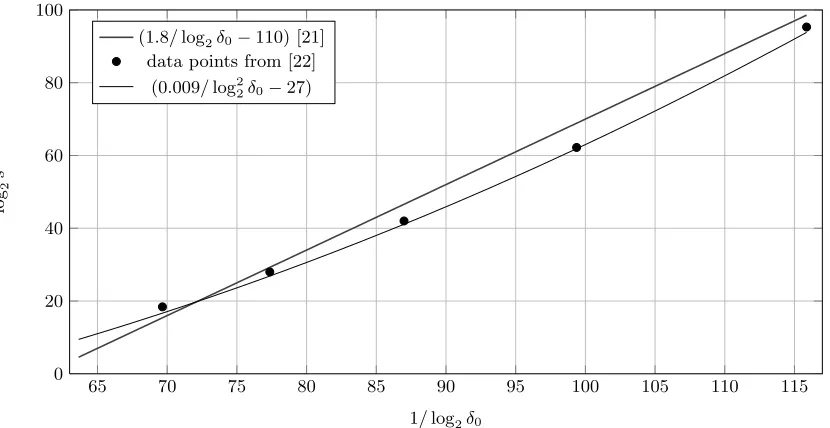
In [12] the authors present a study of ‘BKZ 2.0’, the amalgamation of three folklore techniques to improve the performance of BKZ: pruned enumeration; pre-processing of local blocks and early termination. While no implementations of such algorithms are publicly available, the authors of [12] present a simulator to predict the behaviour of out-of-reach BKZ algorithms. However, the accuracy of this simulator has not been independently verified. In a recent work [22], the authors re-visit the BKZ running-time model of [21] and compare the predictions to the simulator of [12] in a few cases. In the cases examined in [22], the running-time predictions obtained by the use of the BKZ 2.0 simulator are quite close to those obtained by the model of Lindner and Peikert.
Based on the data-points provided in [22] and converting these to the same metric as in the Lindner-Peikert model, the function
log2TsecBKZ2.0= 0.009/log22δ0−27
provides a very close approximation to the running-time output of the simulator for this particular case (cf. Figure 1).
This is a non-linear approximation and hence naturally grows faster than the approximation in [21]. This does not imply that the BKZ 2.0 algorithm is slower than the variant implemented in NTL, as these are two different estimates for the same algorithm (the extrapolation of [21] aimed to take into account the advances collectively known as BKZ 2.0). However, given the greater sophistication of the latter “BKZ 2” extrapola-tions derived from the simulator of [12], we expect this model to provide more accurate approximaextrapola-tions of running times than the model of [21].
In particular, a BKZ logarithmic running-time model which is non-linear in log2(δ0) appears more intuitive than a linear model. While, in practise, the root Hermite factors achievable through the use of BKZ with a particular blocksizeβ are much better than their best provable upper bounds, the root factor achievable appears to behave similarly to the upper bounds as a function ofβ. Namely, the best proven upper bounds on the root Hermite factor are of the form√γβ1/(β−1), where γβ denotes the best known upper bound on the Hermite constant for lattices of dimension β. Now since, asymptotically, γβ grows linearly in β, if we assume that the root Hermite factor achievable in practise displays asymptotic behaviour similar to that of the best-known upper bound, then the root Hermite factor achievable as a function of β, denotedδ0(β), is such that δ0(β)∈ Ω(1/β). Since the running time of BKZ appears to be doubly-exponential in β, we can derive that logTsecis non-linear in 1/log(δ0), as is borne out by the results in [22]. We also note that in [21] the assumption is made that logTsec=O(1/log(δ0)), which does not hold from the above discussion.
Using this model, we can give an analogue of Table 4 in which the BKZ entries are obtained using the above approximate model.
65 70 75 80 85 90 95 100 105 110 115 0
20 40 60 80 100
1/log2δ0
log
2
s
(1.8/log2δ0−110) [21] data points from [22]
(0.009/log22δ0−27)
Fig. 1.BKZ running times in secondssfor given values ofδ0.
n q αq BKW BKZ 2.0 Simulator Model
tlog2mlog2#Zqlog2#Z2 log2#Ls,χ log2log2mlog2#Zqlog2#Z2log2#Ls,χ
Regev [29]
128 16411 11.81 3.2 81.62 93.84 97.65 83.85 -14 22.50 61.90 65.71 22.50 256 65537 25.53 3.1 126.26 179.76 183.76 168.79 -35 44.48 174.46 178.46 44.48 512 262147 57.06 3.1 337.92 350.80 354.97 338.02 -94 104.47 518.62 522.79 104.47
Lindner & Peikert [21]
128 2053 2.70 2.9 63.86 82.40 85.86 72.73 -14 22.28 57.06 60.52 22.28 256 4099 3.34 2.8 105.08 151.45 155.04 140.64 -33 42.21 151.16 154.74 42.21 512 4099 2.90 2.6 157.78 278.01 281.59 266.14 -86 96.09 424.45 428.03 96.09
Table 5. Cost of distinguishing LWE samples from uniform as reported as “Distinguish” in [21], compared to Corollary 3. BKZ estimates obtained using BKZ 2.0 simulator-derived cost estimate.
5.2 Short Integer Solutions: Combinatorial
Recall that if we consider the set of samples from Ls,χ used during the course of the BKW algorithm as determining aq-ary lattice, and the noisy vector as denoting a point close to a lattice point, we may consider the BKW algorithm as analysed in Corollary 3 as a combinatorial approach for sampling a sparseuin the dual lattice with entries∈ {−1,0,1}. Hence, it is related to a combinatorial approach for finding short dual-(q-ary)lattice vectors as briefly sketched in [24, p. 156] (cf. also [23]). These algorithms, however, operate somewhat differently to BKW - given a relatively small set of LWE samples, these are divided into a small number of subsets. Within each subset, we compute all linear combinations of the members of that subset such that the coefficients of these linear combinations are in {−b0, . . . , b0} (note that the parameter b0 is unrelated to the parameterbused in this work).
There are some significant differences between such algorithms and BKW, stemming from the assumption of the former that we only have access to a very small number of LWE samples. This requires the ‘expansion’ of the sample set in such a way that when we search for collisions, we are almost certain to find enough. On the other hand, due to this expansion, the initial samples must be separated into disjoint lists. Thus, probably the easiest way to describe the algorithm in [24] in terms of BKW is to imagine a variant of BKW where, if a sample is not in a given table, we add this sample plus all {−b, . . . , b}-bounded linear combinations of this sample with the pre-existing table entries, to the table. To give a strict analogue to [24], on finding a subsequent collision, we would need to store a list of all noise elements which had been added to a sample and ensure that, if we want to eliminate a sample, that the set of noise elements belonging to the sample and the set of noise elements belonging to the table entry are disjoint.
However, the fundamental difference stems from the assumption that the number of samples is restricted. If this is not the case (as we assume), then it is clear that BKW delivers a much shorter dual lattice vector.
5.3 Bounded Distance Decoding: Lattice Reduction
In [21], the authors propose a method to solve LWE instances which consists ofq-ary lattice reduction, then employing a decoding stage to determine the secret. The decoding stage used is essentially a straightforward modification of Babai’s well-known nearest plane algorithm for CVP. The authors estimate the running-time of the BKZ algorithm in producing a basis ‘reduced-enough’ for the decoding stage of the algorithm to succeed, then add the cost of the decoding stage.
To obtain comparable complexity results, we calculate upper bounds on the bit operation counts for two data-points based on the running times reported in [21] multiplied by the clock speed of the CPU used. As can be seen from Table 6, unsurprisingly these indicate substantially lower complexities than for BKW. In addition, the memory requirements of this approach are small compared to the memory requirements of BKW.
n q αq BKW NTL-BKZ Lindner/Peikert Model
tlog2mlog2#Zqlog2#Z2 log2#Ls,χ log2log2mlog2#Zqlog2#Z2 log2#Ls,χ
136 2003 5.19 2.6 67.49 93.77 97.23 84.15 -25 33.46 91.35 94.81 33.46 214 16381 2.94 3.4 76.90 128.36 132.16 117.54 -18 26.95 82.31 86.11 26.95
Table 6.Cost of solving Search-LWE reported as “Decode” in [21], compared to the cost solving Decision-LWE with BKW
5.4 Bounded Distance Decoding: Combinatorial
We can take the approach of viewing LWE as being the problem of solving BDD in a random q-ary lattice with a random target t=As+e. To solve the LWE problem formulated thus, we have several choices of lattice-based algorithms. However, for several such algorithms, tight complexity estimates are unavailable, thus making comparison to BKW loose. One algorithm for which more precise complexity estimates are available is the AKS (Ajtai, Kumar & Sivakumar) algorithm for solving the shortest vector problem [2]. This algorithm is notable as being the first proposed singly-exponential SVP algorithm.
Subsequent developments of the AKS algorithm by Regev, Nguyen and Vidick, Micciancio and Voulgaris, Pujol and Stehle delivered algorithms which were of time complexity 216n+o(n), 25.9n+o(n), 23.4n+o(n) and 22.7n+o(n), respectively [18].
6
Experimental Results
In order to verify the results of this work, we implemented stages 1 and 2 of the BKW algorithm. Our implementation considers LWE with short secrets but we ignore the transformation cost to produce samples with a short secret. Also, our implementation supports arbitrary bit-width windowsb, not only multiplies of
dlog2(q)e. However, due to the fact that our implementation does not use a balanced representation of finite field elements internally – which simplifies dealing with arbitrary bit-width windows – our implementation does notfullyimplement the half-table improvement. That is, for simplicity, our implementation only uses the additive inverse of a vector if this is trivially compatible with our internal data representation. Furthermore, our implementation does not bit-pack finite field elements. Elements always take up 16 bits of storage. Overall, the memory consumption of our implementation in stage 1 is worse by a factor of up to four compared to the estimates given in this work and the computational work in stage is worse by a factor of up to two. Finally, since our implementation is not optimised we do not report CPU times.
With these considerations in mind, our estimates are confirmed by our implementation. For example, consider Regev’s parameters for n = 25 and t = 2.3 and d = 1, By Lemma 9 picking m = 212.82 will result in a success probability of psuccess ≈0.99959 per component and Psuccess ≈0.99 overall. Lemma 2 estimates a computational cost of 230.54 ring operation and 224.19 calls toL
s,χ in stage 1. We ran our implementation withm=d212.82cand window bitsizew= 22 = nlog2(q)
2.3 log2(n). It required 2
29.74 ring operations and 223.31 calls toLs,χ to recover one component ofs. From this we conclude that Theorem 2 is reasonably tight.
To test the accuracy of Lemma 9 we ran our implementation with the parametersn= 25,q= 631,α·q= 5.85, w= 24 = nlog2(q)
2.1 log2(n) andm= 2
7. Lemma 9 predicts a success rate of 53%. In 1000 experiments we 665 times rank zero for the correct key component, while Lemma 9 predicted 530. Hence, it seems our predictions are slightly pessimistic. The distribution of the ranks of the correct component ofsin 1000 experiments is plotted in Figure 2.
0 1 2 3 4 5 6 7 8 9 10
0 0.2 0.4 0.6 0.8 1
Rank
Coun
t
Fig. 2.Distribution of right key component ranks for 1000 experiments onn= 25,t= 2.3,d= 1, psuccess= 0.99.
7
Conclusion and Further Work
In this work we have provided a concrete analysis of the cost of running the BKW algorithm on LWE instances both for the search and the decision variants of the LWE problem. We also applied this analysis to various sets of parameters found in the literature. From this we conclude that the BKW algorithm outperforms lattice reduction algorithms in an SIS setting for the parameter sets proposed in [29, 21] starting around dimension n ≈ 250 at the cost of requiring many more samples and storage. On the other hand, lattice reduction in a BDD setting currently outperforms the BKW algorithm as analysed in this work.
A pressing research question for future work is hence how to apply a variant of the BKW algorithm to the BDD problem. Furthermore, in this work we ignore the so-called LWE “normal form” where the secret follows the noise distribution χ (cf. [10]) and other small secret variants of LWE. For the BKW algorithm as presented in this work, only hypothesis testing is affected by the size of the secret and hence we do not expect the algorithm to benefit from considering small secrets. Yet, a dedicated variant of the BKW algorithm tackling small secrets is a promising research direction.
Acknowledgements
References
1. Shweta Agrawal, Craig Gentry, Shai Halevi, and Amit Sahai. Discrete Gaussian Leftover Hash Lemma over infinite domains. Cryptology ePrint Archive, Report 2012/714, 2012. http://eprint.iacr.org/.
2. Mikl´os Ajtai, Ravi Kumar, and D. Sivakumar. Sampling short lattice vectors and the closest lattice vector problem. InIEEE Conference on Computational Complexity, pages 53–57, 2002.
3. Martin Albrecht, Carlos Cid, Jean-Charles Faug`ere, Robert Fitzpatrick, and Ludovic Perret. On the complexity of the Arora-Ge algorithm against LWE. InSCC ’12: Proceedings of the 3nd International Conference on Symbolic Computation and Cryptography, pages 93–99, Castro-Urdiales, July 2012.
4. Martin R. Albrecht.bkw-estimator.py, 2012. available athttps://bitbucket.org/malb/research-snippets/. 5. Martin R. Albrecht, Pooya Farshim, Jean-Charles Faug`ere, and Ludovic Perret. Polly Cracker, revisited. In
Advances in Cryptology – ASIACRYPT 2011, volume 7073 of Lecture Notes in Computer Science, pages 179– 196, Berlin, Heidelberg, New York, 2011. Springer Verlag. full version available as Cryptology ePrint Archive, Report 2011/289, 2011http://eprint.iacr.org/.
6. Martin R. Albrecht, Robert Fitzpatrick, Daniel Cabracas, Florian G¨opfert, and Michael Schneider. A generator for LWE and Ring-LWE instances, 2013. available at http://www.iacr.org/news/files/ 2013-04-29lwe-generator.pdf.
7. Sanjeev Arora and Rong Ge. New algorithms for learning in presence of errors. In Luca Aceto, Monika Hen-zinger, and Jiri Sgall, editors,ICALP, volume 6755 ofLecture Notes in Computer Science, pages 403–415, Berlin, Heidelberg, New York, 2011. Springer Verlag.
8. Thomas Baigneres, Pascal Junod, and Serge Vaudenay. How far can we go beyond Linear Cryptanalysis? In Pil Joong Lee, editor,Advances in Cryptology – ASIACRYPT 2004, volume 3329 ofLecture Notes in Computer Science, pages 432–450, Berlin, Heidelberg, New York, 2004. Springer Verlag.
9. Avrim Blum, Adam Kalai, and Hal Wasserman. Noise-tolerant learning, the parity problem, and the statistical query model. J. ACM, 50(4):506–519, 2003.
10. Zvika Brakerski, Adeline Langlois, Chris Peikert, Oded Regev, and Damien Stehl´e. Classical hardness of Learning with Errors. to appear STOC 2013, 2013.
11. Zvika Brakerski and Vinod Vaikuntanathan. Efficient fully homomorphic encryption from (standard) LWE. In Rafail Ostrovsky, editor,IEEE 52nd Annual Symposium on Foundations of Computer Science, FOCS 2011, pages 97–106. IEEE, 2011.
12. Yuanmi Chen and Phong Q. Nguyen. BKZ 2.0: better lattice security estimates. In Advances in Cryptology -ASIACRYPT 2011, volume 7073 of Lecture Notes in Computer Science, pages 1–20, Berlin, Heidelberg, 2011. Springer Verlag.
13. Lutz Duembgen. Bounding standard gaussian tail probabilities. arXiv:1012.2063, 2010.
14. Pierre-Alain Fouque and ´Eric Levieil. An improved LPN algorithm. In Roberto De Prisco and Moti Yung, editors,
Security and Cryptography for Networks, 5th International Conference, SCN 2006, volume 4116 ofLecture Notes in Computer Science, pages 348–359. Springer Verlag, 2006.
15. Nicolas Gama, Phong Q. Nguyen, and Oded Regev. Lattice enumeration using extreme pruning. InAdvances in Cryptology – EUROCRYPT 2010, volume 6110 ofLecture Notes in Computer Science, pages 257–278. Springer Verlag, 2010.
16. Craig Gentry. A fully homomorphic encryption scheme. PhD thesis, Stanford University, 2009. Available at
http://crypto.stanford.edu/craig.
17. Craig Gentry, Chris Peikert, and Vinod Vaikuntanathan. Trapdoors for hard lattices and new cryptographic constructions. In STOC 08: Proceedings of the 40th annual ACM symposium on Theory of computing, pages 197–206. ACM, 2008.
18. Guillaume Hanrot, Xavier Pujol, and Damien Stehl´e. Algorithms for the shortest and closest lattice vector problems. In Yeow Meng Chee, Zhenbo Guo, San Ling, Fengjing Shao, Yuansheng Tang, Huaxiong Wang, and Chaoping Xing, editors, IWCC, volume 6639 ofLecture Notes in Computer Science, pages 159–190. Springer, 2011.
19. Guillaume Hanrot, Xavier Pujol, and Damien Stehl´e. Analyzing blockwise lattice algorithms using dynamical systems. In Phillip Rogaway, editor,Advances in Cryptology – CRYPTO 2011, volume 6841 ofLecture Notes in Computer Science, pages 447–464. Springer Verlag, 2011.
20. Fredrik Johansson et al.mpmath: a Python library for arbitrary-precision floating-point arithmetic (version 0.17), February 2011. http://code.google.com/p/mpmath/.
![Table 1. Cost of solving Search-LWE for parameters suggested in [29] with d = 1, t = 3, ϵ = 0.99 with BKW.](https://thumb-us.123doks.com/thumbv2/123dok_us/7883912.1308122/18.612.183.429.444.637/table-cost-solving-search-lwe-parameters-suggested-bkw.webp)
![Table 3. Cost of finding G ≈ s for parameters suggested in [5] with d = 2, ϵ = 0.99.](https://thumb-us.123doks.com/thumbv2/123dok_us/7883912.1308122/19.612.116.494.185.253/table-cost-nding-g-s-parameters-suggested.webp)
![Table 4. Cost of solving Decision-LWE with BKZ as in [21] and BKW as in Corollary 3.](https://thumb-us.123doks.com/thumbv2/123dok_us/7883912.1308122/20.612.99.514.70.184/table-cost-solving-decision-lwe-bkz-bkw-corollary.webp)
![Table 6. Cost of solving Search-LWE reported as “Decode” in [21], compared to the cost solving Decision-LWE withBKW](https://thumb-us.123doks.com/thumbv2/123dok_us/7883912.1308122/22.612.103.511.429.478/solving-search-reported-decode-compared-solving-decision-withbkw.webp)

