Lower Bounds in the Hardware Token Model
Shashank Agrawal∗ Prabhanjan Ananth† Vipul Goyal‡.
Manoj Prabhakaran§ Alon Rosen¶
Abstract
We study the complexity of secure computation in the tamper-proof hardware token model. Our main focus is on non-interactive unconditional two-party computation using bit-OT to-kens, but we also study computational security with stateless tokens that have more complex functionality. Our results can be summarized as follows:
• We show that there exists a class of functions such that the number of bit-OT tokens required to securely implement them is at least the size of the sender’s input. The same applies for receiver’s input size (with a different class of functionalities).
• We investigate the existence of non-adaptive protocols in the hardware token model. In a non-adaptive protocol, the queries to the tokens are fixed in advance as against an adaptive protocol in which the queries can depend on the answers from the previously queried tokens. In this work, we show that the existence of non-adaptive protocols in the hardware token model imply efficient (decomposable) randomized encodings. Since, efficient decomposable randomized encodings are believed to not exist for all efficient functions, this result can be interpreted as an evidence to the impossibility of non-adaptive protocols for efficiently computable functions.
• We investigate the number of calls to the hardware (which isstateless) required in hardware based obfuscation. By Barak et al., we know that at least one call to the hardware is required. In this work, we show that even with a constant number of calls we cannot realize hardware based obfuscation for all efficient functionalities.
The first two results are in the information-theoretic setting while the last result is in the com-putational setting. En route to proving our results, we make interesting connections between the hardware token model and well studied notions such asOT hybrid model,randomized encodings
andobfuscation.
∗
University of Illinois Urbana-Champaign. Email: [email protected]. Part of this work was done at Microsoft Research India. Research supported in part by NSF grants 1228856 and 0747027.
†
University of California Los Angeles. Email: [email protected]. Part of this work was done at Microsoft Research India and part of this work was done while visiting IDC Herzliya, supported by the ERC under the EU’s Seventh Framework Programme (FP/2007-2013) ERC Grant Agreement n. 307952
‡
Microsoft Research, India. Email: [email protected]
§
University of Illinois Urbana-Champaign. Email: [email protected]. Research supported in part by NSF grants 1228856 and 0747027.
¶
1
Introduction
A protocol for secure two-party computation allows two mutually distrustful parties to jointly compute a function f of their respective inputs, x and y, in a way that does not reveal anything beyond the value f(x, y) being computed. Soon after the introduction of this powerful notion [46,
22], it was realized that most functionsf(x, y) do not admit an unconditionally-secure protocol that satisfies it, in the sense that any such protocol implicitly implies the existence (and in some case requires extensive use [2]) of a protocol for Oblivious Transfer (OT) [10, 3,33,27,39]. Moreover, even if one was willing to settle for computational security, secure two-party computation has been shown to suffer from severe limitations in the context of protocol composition [19,7,36,37].
The above realizations have motivated the search for alternative models of computation and communication, with the hope that such models would enable bypassing the above limitations, and as a byproduct perhaps also give rise to more efficient protocols. One notable example is the so calledhardware token model, introduced by Katz [32]. In this model, it is assumed that one party can generate hardware tokens that implement some efficient functionality in a way that allows the other party only black-box access to the functionality.
The literature on hardware tokens (sometimes referred to as tamper prooftokens1) discusses a variety of models, ranging from the use of stateful tokens (that are destroyed after being queried for some fixed number of times) to stateless ones (that can be queried for an arbitrary number of times), with eithernon-adaptiveaccess (in which the queries to the tokens are fixed in advance) or adaptiveaccess (in which queries can depend on answers to previous queries). Tokens with varying levels of complexity have also been considered, starting with simple functions such as bit-OT, and ranging all the way to extremely complex functionalities (ones that enable the construction of UC-secure protocols given only a single call to the token).
The use of hardware tokens opened up the possibility of realizing information-theoretically and/or composable secure two-party protocols even in cases where this was shown to be impossible in “plain” models of communication. Two early examples of such constructions are protocols for UC-secure computation [32], and one-time programs [24]. More recently, a line of research initiated by Goyal et al. [26] has focused on obtaining unconditionally-secure two-party computation using stateful tokens that implement the bit-OT functionality. In [25], Goyal et al. went on to show how to achieve UC-secure two party computation using stateless tokens under the condition that tokens can be encapsulated: namely, the receiver of a token A can construct a token B that can invoke A internally. Finally, Dottling et al. [16] have shown that it is possible to obtain information-theoretically secure UC two-party protocols using a single token, assuming it can compute some complex functionality.
Generally speaking, the bit-OT token model has many advantages over a model that allows more complex tokens. First of all, the OT functionality is simple thus facilitating hardware design and implementation. Secondly, in many cases [26], the bit-OT tokens do not depend on the functionality that is being computed. Hence, a large number of bit-OT tokens can be produced “offline” and subsequently used for any functionality. The main apparent shortcoming of bit-OT tokens in comparison to their complex counterparts is that in all previous works the number of tokens used is proportional to the size of the circuit being evaluated, rendering the resulting protocols impractical. This state of affairs calls for the investigation of the minimal number of bit-OT token invocations in a secure two-party computation protocol.
1
In this work we aim to study the complexity of constructing secure protocols with respect to different measures in the hardware token model. Our main focus is on non-interactive information-theoretic two-party computation using bit-OT tokens, but we also study computational security with stateless tokens that compute more complex functionalities. En route to proving our results, we make interesting connections between protocols in the hardware token model and well studied notions such as randomized encodings, obfuscation and the OT hybrid model. Such connections have been explored before mainly in the context of obtaining feasibility results [26,17].
The first question we address is concerned with the number of bit-OT tokens required to securely achieve information-theoretic secure two-party computation. The work on one-time programs makes use of bit-OT tokens in order to achieve secure two party computation in the computational setting, and the number of tokens required in that construction is proportional to the receiver’s input size. On the other hand, the only known construction in the information-theoretic setting [26] uses a number of tokens that is proportional to the size of the circuit. This leads us to the following question: is it possible to construct information theoretic two party computation protocols in the token model, where the number of tokens is proportional to the size of the functionality’s input? Problems of similar nature have been also studied in the (closely related) OT-hybrid model [15,2,45,41,42,44].
The second question we address is concerned with the number of levels of adaptivity required to achieve unconditional two party computation. The known constructions [26] using bit-OT tokens are highly adaptive in nature: the number of adaptive calls required is proportional to the depth of the circuit being computed. The only existing protocols which are non-adaptive are either for specific complexity classes ([30] for NC1) or in the computational setting [24]. An interesting question, therefore, is whether there exist information-theoretic non adaptive protocols for all efficient functionalities.
The works of [25, 38] give negative results on the feasibility of using stateless tokens in the information-theoretic setting. Goyal et al. [26] have shown that it is feasible to construct proto-cols using stateless tokens under computational assumptions. So, a natural question would be to determine the minimum number of calls to the (stateless) token required in a computational setting.
1.1 Our Results
We exploit the relation between protocols in the hardware token model and cryptographic notions such as randomized encodings and obfuscation to obtain lower bounds in the hardware token model. We focus on non-interactive two-party protocols, where only one party (the sender) sends messages and tokens to the other party (the receiver). Our results are summarized below.
Number of bit-OT tokens in the information-theoretic setting. Our first set of results
establishes lower bounds on the number of bit-OT tokens as a function of the parties’ input sizes. Specifically:
• We show that there exists a class of functionalities such that the number of tokens required to securely implement them is at least the size of the sender’s input. To obtain this result, we translate a similar result in the correlated distributed randomness model by Winkler et al. [44] to this setting.
While this still leaves a huge gap between the positive result (which uses number of tokens proportional to the size of the circuit) and our lower bound, we note that before this result, even such lower bounds were not known to exist. Even in the case of OT-hybrid model, which is very much related to the hardware token model (and more deeply studied), only lower bounds known are in terms of the sender’s input size.
Non-adaptive protocols and randomized encodings. In our second main result we show
that non-adaptive protocols in the hardware token model imply efficient randomized encodings. Even though currently known protocols [26] are highly adaptive, it was still not clear that non adaptive protocols for all functionalities were not possible. In fact, all functions in NC1 admit non adaptive protocols in the hardware token model [30]. To study this question, we relate the existence of non-adaptive protocols to the existence of a “weaker” notion of randomized encodings, called decomposable randomized encodings. Specifically, we show that if a function has a non adaptive protocol then correspondingly, the function has an efficient decomposable randomized encoding. The existence of efficient decomposable randomized encodings has far-reaching implications in MPC, providing strong evidence to the impossibility of non-adaptive protocols for a large class of functions.
Constant number of calls to stateless tokens. In our last result we show that there exists
a functionality for which there does not exist any protocol in the stateless hardware token model making at most a constant number of calls. To this end, we introduce the notion of an obfuscation complete oracle scheme, a variant of obfuscation tailored to the setting of hardware tokens. Goyal et. al. [26] have shown such a scheme can be realized under computational assumptions (refer to Section 6.2.2 in the full version). We derive a lower bound stating that a constant number of calls to the obfuscation oracle does not suffice. This can be seen as a strengthening of the impossibility result by Barak et al. [1] which states that at least one call to the obfuscation oracle is required. This result can then be translated to a corresponding result in the hardware token model. This result holds even if the hardware is a complex stateless token (and hence still relevant even in light of our previous results) and (more importantly) against computational adversaries. Previous known lower bounds on complex tokens were either for the case of stateful hardware [23,24,18] or in the information theoretic setting [25,38].
Our hope is that the above results will inspire future work on lower bounds in more general settings in the hardware token model and to further explore the connection with randomized en-codings, obfuscation and the OT-hybrid model.
1.2 Related Work
computation where only one partyGoliath is capable of generating tokens. Damgard et al. [13,14] weaken the ‘isolation’ assumption of Katz; they allow a token to communicate a fixed number of bits to its creator.
Goyal et al. [26] construct the first unconditionally secure protocol for arbitrary functionalities using stateful tokens. Their protocol is non-interactive and only one party obtains the output of the computation. They also construct a general purpose obfuscation scheme from stateless tokens. In [25], Goyal et al. provide several interesting results about the power of stateless tokens. They show that such tokens can be used to construct statistically secure commitment protocols and zero-knowledge proofs forNP. They also show that if one token can be encapsulated into another, an unconditionally secure protocol exists for any functionality. Furthermore, if this encapsulation is not possible, then statistically secure oblivious transfer cannot be realized. Dottling et al. [16] show that information-theoretic UC-secure two party computation is achievable with the help of just one tamper-proof device. In [18], Dottling et al. study how general resettable computation can be realized using one (or two) stateless tokens and minimal number of rounds of interaction.
2
Preliminaries
2.1 Model of computation
Hardware tokens: Hardware tokens can be divided into two broad categories – stateful and
stateless. As the name implies, stateful tokens can maintain some form of state, which might restrict the extent to which they can be used. On the other hand, stateless tokens cannot maintain any state, and could potentially be used an unbounded number of times. The first formal study of hardware tokens modeled them as stateful entities [32], so that they can engage in a two-round protocol with the receiver. Later on, starting with the work of Chandran et al. [8], stateless tokens were also widely studied.
The token functionality models the following sequence of events: (1) a player (the creator) ‘seals’ a piece of software inside a tamper-proof token; (2) it then sends the token to another player (the receiver), who can run the software in a black-box manner. Once the token has been sent, the creator cannot communicate with it, unlike the setting considered in [13,14]. We also do not allow token encapsulation [25], a setting in which tokens can beplaced inside other tokens.
Stateless tokens: The Fstateless
wrap functionality models the behavior of a stateless token. It is
parameterized by a polynomialp(.) and an implicit security parameterk. Its behavior is described as follows:
• Create: Upon receiving (create,sid, Pi, Pj,mid, M) from Pi, where M is a Turing machine,
do the following: (a) Send (create,sid, Pi, Pj,mid) to Pj, and (b) Store (Pi, Pj,mid, M).
• Execute: Upon receiving (run,sid, Pi,mid,msg) fromPj, find the unique stored tuple (Pi, Pj,
mid, M). If no such tuple exist, do nothing. RunM(msg) for at mostp(k) steps, and letout
be the response (out=⊥ifM does not halt inp(k) steps). Send (sid, Pi,mid,out) to Pj.
Here sidand middenote the session and machine identifier respectively.
studied primitives in secure multi-party computation. In the nt
-OTk variant, sender hasnstrings of k bits each, out of which a receiver can pick any t. The sender does not learn anything in this process, and the receiver does not know what the remaining n−tstrings were. The behavior of an OTM token is similar to 21
-OTk.
The primary difference between the OT functionality and an OTM token is that while the functionality forwards an acknowledgment to the sender when the receiver obtains the strings of its choice, there is no such feedback provided by the token. Hence, one has to put extra checks in a protocol (in the token model) to ensure that the receiver opens the tokens when it is supposed to (see, for example, Section 3.1 in [26]). Formal definitions of FOT andFOT M are given below. We
would be dealing with OTMs where both inputs are single bits. We will refer to them as bit-OT tokens.
Oblivious Transfer (OT): The functionality FOT is parameterized by three positive integers n,
tand k, and behaves as follows.
• On input (Pi, Pj,sid,id,(s1, s2, . . . , sn)) from partyPi, send (Pi, Pj,sid,id) toPj and store the
tuple (Pi, Pj,sid,id,(s1, s2, . . . , sn)). Here eachsi is a k-bit string.
• On receiving (Pi,sid,id, l1, l2, . . . , lt) from party Pj, if a tuple (Pi, Pj,sid,id, (s1, s2, . . . , sn))
exists, return (Pi,sid,id, sl1, sl2, . . . , slt) to Pj,send an acknowledgment(Pj,sid,id) to Pi, and delete the tuple (Pi, Pj,sid,id,(s1, s2, . . . , sn)). Else, do nothing. Here each lj is an
integer between 1 and n.
One Time Memory (OTM): The functionalityFOT M which captures the behavior an OTM is
described as follows:
• On input (Pi, Pj,sid,id,(s0, s1)) from party Pi, send (Pi, Pj,sid,id) to Pj and store the tuple
(Pi, Pj,sid,id,(s0, s1)).
• On receiving (Pi,sid,id, c) from party Pj, if a tuple (Pi, Pj,sid,id,(s0, s1)) exists, return
(Pi,sid,id, sc) toPj and delete the tuple (Pi, Pj,sid,id,(s0, s1)). Else, do nothing.
Non-interactivity: In this paper, we are interested in non-interactive two-party protocols (i.e., where only one party sends messages and tokens to the other). Some of our results, however, hold for an interactive setting as well (whenever this is the case, we point it out). The usual setting is as follows: Alice and Bob have inputs x ∈ Xk and y ∈ Yk respectively, and they wish to securely
compute a functionf :Xk× Yk→ Zk, such that only Bob receives the outputf(x, y)∈ Zk of the computation (here,kis the security parameter). Only Alice is allowed to send messages and tokens to Bob.
Circuit families. In this work, we assume that parties are represented by circuit families instead of Turing machines. A circuit is an acyclic directed graph, with the gates of the circuit representing the nodes of the graph, and the wires representing the edges in the graph. A circuit can either be boolean or arithmetic depending on whether the gates are AND-OR or ADD-MULTIPLY gates. We assume that the circuit can be broken down into layers such that the first layer takes the input of the circuit and outputs to the second layer and so on. The output of the last layer is the output of the circuit.
denoted byDepth(C) to be the number of layers in the circuit. There are several complexity classes defined in terms of depth and size of circuits. One important complexity class that we will refer in this work is the NC1 complexity class. This comprises of circuits which have depth O(log(n)) and sizepoly(n), where nis the input size of the circuit. Languages in P can be represented by a circuit family whose size is polynomial in the size of the input.
2.2 Security
Definition 1(Indistinguishability). A functionf :N→Ris negligible in nif for every polynomial
p(.)and all sufficiently largen’s, it holds thatf(n)< p(1n). Consider two probability ensemblesX :=
{Xn}n∈N and Y := {Yn}n∈N. These ensembles are computationally indistinguishable if for every PPT algorithm A, |Pr[A(Xn,1n) = 1]−Pr[A(Yn,1n) = 1]| is negligible in n. On the other hand,
these ensembles are statistically indistinguishable if∆(Xn, Yn) = 12Pα∈S|Pr[Xn=α]−Pr[Yn=α]|
is negligible inn, whereS is the support of the ensembles. The quantity∆(Xn, Yn) is known as the
statistical difference between Xn andYn.
Statistical security: A protocol π for computing a two-input function f :Xk× Yk → Zk in the
hardware-token model involves Alice and Bob exchanging messages and tokens. In the (static) semi-honest model, an adversary could corrupt one of the parties at the beginning of an execution of π. Though the corrupted party does not deviate from the protocol, the adversary could use the information it obtains through this party to learn more about the input of the other party. At an intuitive level, a protocol is secure if any information the adversary could learn from the execution can also be obtained just from the input and output (if any) of the corrupted party. Defining security formally though requires that we introduce some notation, which we do below.
Let the random variables viewπA(x, y) = (x, RA, M, U) and viewπB(x, y) = (y, RB, M, V) denote
the views of Alice and Bob respectively in the protocol π, when Alice has input x ∈ Xk and Bob
has input y ∈ Yk. Here RA (resp. RB) denotes the coin tosses of Alice (resp. Bob), M denotes
the messages exchanged between Alice and Bob, andU (resp. V) denotes the messages exchanged between Alice (resp. Bob) and the token functionality. Also, let outπ
B(x, y) denote the output
produced by Bob. We can now formally define security as follows.
Definition 2(-secure protocol [44]). A two-party protocolπcomputes a functionf :Xk×Yk → Zk
with−security in the semi-honest model if there exists two randomized functionsSA andSB such
that for all sufficiently large values ofk, the following two properties hold for allx∈ Xk andy∈ Yk:
• ∆((SA(x), f(x, y)),(viewπA(x, y),outπB(x, y)))≤(k),
• ∆(SB(y, f(x, y)),viewπB(x, y))≤(k).
If π computes f with -security for a negligible function (k), then we simply say that π securely
computes f. Further if(k) = 0, π is aprefectly secure protocol for f.
Information Theory: We define some information-theoretic notions which will be useful in prov-ing unconditional lower bounds. Entropy is a measure of the uncertainty in a random variable. The entropy of X given Y is defined as:
H(X|Y) =−X
x∈X X
y∈Y
For the sake of convenience, we sometimes use h(p) = −plogp−(1−p) log(1−p) to denote the entropy of a binary random variable which takes value 1 with probabilityp (0≤p≤1).
Mutual information is a measure of the amount of information one random variable contains about another. The mutual information between X and Y given Z is defined as follows:
I(X;Y|Z) =H(X|Z)−H(X|Y Z).
See [11] for a detailed discussion of the notions above.
3
Lower Bounds in Input Size for Unconditional Security
In this section, we show that the number of simple tokens required to be exchanged in a two-party unconditionally secure function evaluation protocol could depend on the input size of the parties. We obtain two bounds discussed in detail in the sections below. Our first bound relates the number of hardware tokens required to compute a function with the input size of the sender. (This bound holds even when the protocol is interactive.) In particular, we show that the number of bit-OT tokens required for oblivious transfer is at least the sender’s input size (minus one). Our second result provides a class of functions where the number of bit-OT tokens required is at least the input size of the receiver.
3.1 Lower bound in Sender’s input size
In this subsection we considerkto be fixed, and thus omitkfromXk,Ykand(k) for clarity. In [44], Winkler and Wullschleger study unconditionally secure two-party computation in the semi-honest model. They consider two parties Alice and Bob, with inputs x∈ X and y ∈ Y respectively, who wish to compute a functionf :X × Y → Z such that only Bob obtains the outputf(x, y)∈ Z (but Alice and Bob can exchange messages back and forth). The parties have access to a functionality
Gwhichdoes not take any input, but outputs a sample (u, v) from a distributionpU V. Winkler and
Wullschleger obtain several lower bounds on the information-theoretic quantities relatingU and V
for a secure implementation of the function f.
Here, we would like to obtain the minimum number of bit-OT tokens required for a secure realization of a function. The functionality which models the token behaviorFOT M is an interactive
functionality: not only does FOT M give output to the parties, but also take inputs from them.
Therefore, as such the results of [44] are not applicable to our setting. However, if we let U
denote all the messages exchanged between Alice and G, and similarly let V denote the entire message transcript between Bob and G, we claim that the following lower bound (obtained for a non-interactive G in [44]) holds even when the functionality G is interactive. This will allow us to apply this bound on protocols where hardware tokens are exchanged.
Theorem 1. Let f :X × Y → Z be a function such that
∀x6=x0 ∈ X ∃y∈ Y :f(x, y)6=f(x0, y).
If there exists a protocol that implementsf from a functionalityG withsecurity in the semi-honest model, then
H(U|V)≥maxy∈YH(X|f(X, y))−(3|Y| −1)(log|Z|+h())−log|X |,
Proof. In order to prove that Theorem 1 holds with an interactive G, we observe that the proof provided by Winkler and Wullschleger for a non-interactiveGalmost goes through for an interactive one. An important fact they use in their proof is that for any protocol π, with access to a non-interactive G, the following mutual information relation holds: I(X;V Y|U M) = 0, where M
denotes the messages exchanged in the protocol. (In other words, X −U M −V Y is a Markov chain.) If one can show that the aforementioned relation holds even whenG can take inputs from the parties (andU andV are redefined as discussed above), the rest of the proof goes through, as can be verified by inspection. Hence, all that is left to do is to prove that I(X;V Y|U M) = 0 is true in the more general setting, where U and V stand for the transcriptsof interactions withG.
We will need the following simple chain rule about mutual information (for a proof see [11]):
I(AA0;B|C) =I(A;B|C) +I(A0;B|AC). (1)
In particular, this implies the following:
I(A;B|CD) =I(A;BC|D)−I(A;C|D) (2)
=I(AC;B|D)−I(B;C|D) (3)
Our goal is to show that the mutual information between X and V Y conditioned on U M is 0. We prove this result with the help of induction on the steps in a protocol. At the beginning of the protocol when no messages have been exchanged (U,V and M are empty random variables),
I(X;V Y|U M) simply becomesI(X;Y). Since we can assume that the inputs of Alice and Bob are chosen independently of each other,I(X;Y) = 0. This proves the base case.
Suppose that the protocol has executed foristeps. Let the messages exchanged up to the firsti
steps between Alice and Bob be denoted byMi, that between Alice andGbyUi, and that between Bob andG byVi. By the induction hypothesis, we know thatI(X;ViY|UiMi) = 0. At thei+ 1th step one of the following things can happen: Alice sends a message to Bob, or vice versa; Alice sends a message to G, or vice versa; Bob sends a message to G, or vice versa. Accordingly, one of the random variables above gets updated. We prove that I(X;Vi+1Y|Ui+1Mi+1) = 0 for some of the updates, and the rest will follow in a similar manner:
• Alice sends a message to G: In this case, Vi+1 =Vi and Mi+1 =Mi. Let the message sent be denoted by Ui+1. Now,
I(X;ViY|Ui+1Mi) =I(X;ViY|UiUi+1Mi)
=I(XUi+1;ViY|UiMi)−I(ViY;Ui+1|UiMi)
=I(X;ViY|UiMi) +I(Ui+1;ViY|XUiMi)
−I(ViY;Ui+1|UiMi),
where the second equality follows from (3), and the third from (1). We know thatI(X;ViY| UiMi) = 0 by the induction hypothesis. Moreover, since Ui+1 is a message sent by Alice,
it is a function of X, Ui and Mi (and the local randomness of Alice). Therefore, ViY → XUiMi → Ui+1, or I(Ui+1;ViY|XUiMi) = 0. Now since mutual information is a positive
• G sends a message to Bob: In this case, Ui+1 =Ui and Mi+1 = Mi. Let the message sent be denoted by Vi+1. Now,
I(X;Vi+1Y|UiMi) =I(X;ViVi+1Y|UiMi)
=I(X;ViY|UiMi) +I(X;Vi+1|UiMiViY)
=I(X;ViY|UiMi) +I(XMiY;Vi+1|UiVi)
−I(Vi+1;MiY|UiVi),
where the second equality follows from (1), and the third from (3). We know thatI(X;ViY| UiMi) = 0 by the induction hypothesis. Moreover, since Vi+1 is a message sent by G, it is a
function of Ui and Vi (and the local randomness of G if any). Therefore, XMiY →UiVi →
Vi+1, or I(XMiY;Vi+1|UiVi) = 0. Now since mutual information is a positive quantity, I(X;Vi+1Y|UiMi) must be 0.
• Bob sends a message to Alice: In this case,Ui+1=Ui and Vi+1 =Vi. Let the message sent be denoted by Mi+1. Now,
I(X;ViY|UiMi+1) =I(X;ViY|UiMiMi+1)
=I(X;ViY Mi+1|UiMi)−I(X;Mi+1|UiMi)
=I(X;ViY|UiMi) +I(X;Mi+1|UiMiViY)
−I(X;Mi+1|UiMi)
=I(X;Mi+1|UiMiViY)−I(X;Mi+1|UiMi)
=I(XUi;Mi+1|MiViY)−I(Mi+1;Ui|MiViY)
−I(X;Mi+1|UiMi),
where the second equality follows from (2), the third from (1), the fourth by the induction, and the fifth by (3). SinceMi+1 is a message sent by G, it is a function of Mi,Vi and Y (and the
local randomness of Bob). Therefore,XUi →MiViY →Mi+1, orI(XUi;Mi+1|MiViY) = 0.
Now since mutual information is a positive quantity,I(X;ViY|UiMi+1) must be 0.
We can handle rest of the events in a similar fashion. This completes the proof ofTheorem 1.
Theorem 1 lets us bound the number of tokens required to securely evaluate a function, as follows. Suppose Alice and Bob exchange`bit-OT tokens during a protocol. If Bob is the recipient of a token, there is at most one bit of information that is hidden from Bob after he has queried the token. On the other hand, if Bob sends a token, he does not know what Alice queried for. Therefore given V, entropy ofU can be at most ` (or H(U|V)≤`). We can use this observation along with Corollary 3 in [44] (full version) to obtain the following result.
Theorem 2. If a protocol-securely realizesmindependent instances of nt-OTk, then the number of bit-OT tokens `exchanged between Alice and Bob must satisfy the following lower bound:
We conclude this section with a particular case of the above theorem which gives a better sense of the bound. Let us say that Alice has a string ofn bits, and Bob wants to pick one of them. In other words, Alice and Bob wish to realize an instance of n1-OT1. Also, assume that they want to do this with perfect security, i.e., = 0. In this case, the input size of Alice is n, but Bob’s input size is onlydlogne. Now, we have the following corollary.
Corollary 3. In order to realize the functionality n1
-OT1 with perfect security, Alice and Bob must exchange at leastn−1 tokens.
Suppose Alice is the only party who can send tokens. Then, we can understand the above result intuitively in the following way. Alice has nbits, but she wants Bob to learn exactly one of them. However, since she does not know which bit Bob needs, she must send her entire input (encoded in some manner) to Bob. Suppose Alice sends `bit-OT tokens to Bob. Since Bob accesses every token, the ` bits it obtains from the tokens should give only one bit of information about Alice’s input. The remaining ` positions in the tokens, which remain hidden from Bob, must contain information about the remainingn−1 bits of Alice’s input. Hence, `must be at leastn−1.
One can use Protocol 1.2 in [5] to show that the bound inCorollary 3is tight.
3.2 Lower bound in Receiver’s input size
In this section, we show that the number of bit-OT tokens required could depend on the receiver’s input size. We begin by defining a non-replayable function family, for which we shall show that the number of tokens required is at least the input size of the receiver.
Definition 3. Consider a function familyf :Xk× Yk→ Zk,k∈I+. We say thatf is replayable if for every distributionDk overXk, there exists a randomized algorithmSB and a negligible function
ν, such that on input (k, y, f(x, y))where (x, y)← Dk× Yk,SB outputs⊥ with probability at most 3/4, and otherwise outputs (y0, z) such that (conditioned on not outputting ⊥) with probability at least 1−ν(k), y0 =6 y and z=f(x, y0).
Theorem 4. Let f : Xk× Yk → Zk be a function that is not replayable. Then, in any
non-interactive protocol π that securely realizes f in the semi-honest model using bit-OT tokens, Alice must send at least n(k) =blog|Yk|c tokens to Bob.
Proof. For simplicity, we omit the parameterkin the following. Suppose Alice sends onlyn−1 bit-OT tokens to Bob in the protocolπ. We shall show thatf is in fact replayable, by constructing an algorithmSB as inDefinition 3, from a semi-honest adversaryAthat corrupts Bob in an execution of π.
Let the input of Alice and Bob be denoted by x and y respectively, where x is chosen from
X according to the distribution D, and y is chosen uniformly at random over Y. On input x, Alice sends tokens (Υ1,· · ·,Υn−1) and a message m to Bob. Bob runs his part of the protocol
with inputs y, m, a random tape r, and (one-time) oracle access to the tokens. Without loss of generality, we assume that Bob queries all the n−1 tokens. Bob’s view consists of y, m, r, and the bits b = (b1, . . . , bn−1) received from the n−1 tokens (Υ1, . . . ,Υn−1). Let q = (q1, . . . , qn−1)
denote the query bits that Bob uses for then−1 tokens. For convenience, we shall denote the view of Bob as (y, m, r, q, b) (even though q is fully determined by the rest of the view).
We define SB as follows: on input (y1, z1), it samples a view (y, r, m, q, b) for Bob in an
(y0, r0, m0, q0, b0) conditioned on (m0, q0, b0) = (m, q, b). If y0 = y, it outputs ⊥. Else, it computes Bob’s output z0 in this execution and outputs (y0, z0).
To argue thatSBmeets the requirements inDefinition 3, it is enough to prove that whenx∈ X
is sampled from any distributionD,y← Y is chosen uniformly, andz=f(x, y): (1) (y0, r0, m0, q0, b0) sampled by SB(y, z) is distributed close (up to a negligible distance) to Bob’s view in an actual execution with inputs (x, y0), and (2) with probability at least 14,y0 6=y. Then, by the correctness of
π, with overwhelming probability, wheneverSBoutputs (y0, z0), it will be the case thatz0=f(x, y0), and this will happen with probability at least 1/4.
The first claim follows by the security guarantee and the nature of a token-based protocol. Consider the experiment of sampling (x, y) and then sampling Bob’s view (y, r, m, q, b) conditioned on input beingyand output beingz=f(x, y). Firstly, this is only negligibly different from sampling Bob’s view from an actual execution ofπ with inputsx andy, since by the correctness guarantee, the output of Bob will indeed be f(x, y) with high probability. Now, sampling (x, y, r, m, q, b) in the actual execution can be reinterpreted as follows: first sample (m, q, b), and then conditioned on (m, q, b), sample x and (y, r) independent of each other. This is because, by the nature of the protocol, conditioned on (m, q, b), Bob’s view in this experiment is independent of x. Now, (y0, r0) is also sampled conditioned on (m, q, b) in the same manner (without resampling x), and hence (x, y0, r0, m, q, b) is distributed as in an execution of π with inputs (x, y0).
To show that SB outputs⊥with probability at most 34, we rely on the fact that the number of distinct inputsy for Bob is 2n, but the number of distinct queries the Bob can make to the tokens
q is at most 2n−1. Below, we fix an (m, b) pair sampled by SB, and argue that Pr[y = y0] ≤ 34
(where the probabilities are all conditioned on (m, b)).
For each value of q ∈ {0,1}n−1 that has a non-zero probability of being sampled by S
B, we
associate a valueY(q)∈ {0,1}nasY(q) = argmax
yPr[y|q], where the probability is over the choice
of y← Y and the random tape r for Bob. If more than one value ofy attains the maximum,Y(q) is taken as the lexicographically smallest one. LetY∗ ={y|∃q s.t. y =Y(q)}. Then,|Y∗| ≤ |Y|/2, or equivalently (since the distribution over Y is uniform), Pr[y 6∈ Y∗]≥ 12.
Let Q∗ ={q|Pr[Y(q)|q]> 12}. Further, let β = min{Pr[Y(q)|q]|q ∈ Q∗}. Note that β > 12. We claim thatα:= Pr[q ∈ Q∗]≤ 1
2. This is because
1
2 ≤Pr[y6∈ Y
∗] = X
y6∈Y∗,q∈Q∗
Pr[y, q] + X
y6∈Y∗,q6∈Q∗
Pr[y, q]
≤ X
q∈Q∗
(1−β) Pr[q] + X
q6∈Q∗
βPr[q] =α(1−β) +β(1−α)
Since β > 12, ifα > 12 then α(1−β) +β(1−α)< 12, which is a contradiction. Hence α≤ 12. Now,
Pr[y=y0]≤αPr[y=y0|q ∈ Q∗] + (1−α) Pr[y=y0|q 6∈ Q∗]
≤α+ (1−α)1 2 ≤
3 4.
We give a concrete example of a function family that is not replayable. Let Xk ={1,2, . . . , k}
be the set of first k positive integers. Let Yk = {S ⊆ Xk : |S| = k/2∧ 1 ∈ S}. Define
Fix a value ofk. Suppose a simulator SB is givenS and f(X, S) as inputs, whereX, S denote random variables uniformly distributed over Xk and Yk respectively. From this input, SB knows that X could take one of k/2 possible values. Any S0 6= S intersects S0 or its complement in at mostk/2−1 positions. Hence,SBcan guess the value of f(X, S0) with probability at most 1−2/k. This implies that if SB outputs (S0, Z) with probability 1/4, with a non-negligible probability
Z 6=f(X, S0).
Note that the number of bits required to represent an element of Xk is only dlogke, but that required to represent an element ofYk is n(k) =dlog12 k/k2
e, which is at least a polynomial ink. Sincef is not replayable, it follows fromTheorem 4that in any protocol that realizesf, Alice must send at least n(k) tokens to Bob.
4
Negative Result for Non-Adaptive Protocols
4.1 Setting
In this section, we explore the connection between the randomized encodings of functions and the protocols for the corresponding functionalities 2 in the bit-OT (oblivious transfer) token model. We deal with only protocols which are non-adaptive, non-interactive and are perfectly secure. The notions of non-interactivity (Section 2.1) and perfect security (Definition 2 in Section 2.2) have already been dealt with in the preliminaries. We will only explain the notion of non-adaptivity. A protocol in the bit-OT token model is said to benon-adaptive if the queries to the tokens are fixed in advance. This is in contrast with the adaptive case where the answers from one token can used to generate the query to the next token.
Such (non-adaptive and non-interactive) protocols have been considered in the literature and one-time programs [24, 26] is one such example, although one-time programs deal with malicious receivers. Henceforth, when the context is clear we will refer to “perfectly secure non-adaptive non-interactive protocols” as just “non-adaptive protocols”.
We show that the existence of non-adaptive protocols for a function in the bit-OT token model implies an efficient (polynomial sized) decomposable randomized encoding for that function. This is done by establishing an equivalence relation between decomposable randomized encodings and a specific type of non-adaptive protocols in the bit-OT token model. Then, we show that a function-ality having any non-adaptive protocol also has this specific type of protocol thereby showing the existence of a DRE for this functionality. Since decomposable randomized encodings are believed to not exist for all functions in P [21,43,20,31], this gives a strong evidence to the fact that there cannot exist non-adaptive protocols in the bit-OT token model for all functions in P.
4.2 Randomized Encodings
We begin this section by describing the necessary background required to understand randomized encodings [29]. A randomized encoding for a function f consists of two procedures - encode and decode. The encode procedure takes an input circuit for f, x which is to the input to f along with randomness r and outputs ˆf(x;r). The decode procedure takes as input ˆf(x;r) and outputs
f(x). There are two properties that the encode and decode procedures need to satisfy for them to
2
qualify to be a valid randomized encoding. The first property is (perfect) correctness which says that the decode algorithm always outputsf(x) when input ˆf(x;r). The second property, namely (perfect) privacy, says that there exists a simulator such that the output distribution of the encode algorithm on input x is identical to the output distribution of the simulator on inputf(x).
We deal with a specific type of randomized encodings termed as decomposable randomized encodings [34,21,28,30,35] which are defined as follows.
Definition 4. An (efficient) Decomposable Randomized Encoding, denoted by DRE, consists of
three PPT algorithms (RE.Encode,RE.ChooseInpWires,RE.Decode):
1. RE.Encode: takes as input a circuitCand outputs( ˜C,state),wherestate= ((s01, s11), . . . ,(s0m, s1m)) and m is the input size of the circuit.
2. RE.ChooseInpWires: takes as input (state, x) and outputs x˜, where x is of length m and x˜= (sx1
1 , . . . , sxmm) and xi is the ith bit of x.
3. RE.Decode: takes as input( ˜C,x˜) and outputs out.
A decomposable randomized encoding needs to satisfy the following properties.
(Correctness):- Let RE.Encode on input C output ( ˜C,state). Let RE.ChooseInpWires on input (state, x) output ˜x. Then,RE.Decode( ˜C,x˜) always outputsC(x).
(Perfect privacy):- There exists a PPT simulator Sim such that the following two distributions are identical.
• n( ˜C,x˜) o
, where ( ˜C,state) is the output of RE.Encode on input C and ˜x is the output of
ChooseInpWires on input (state, x).
• n( ˜CSim,x˜Sim) o
, where ( ˜CSim,x˜Sim) is the output of the simulator Simon input C(x).
In the above definition, -privacy can also be considered instead of perfect privacy where the distributions are far from each other for some negligible . In this section, we only deal with DRE with perfect privacy. It can be verified that a decomposable randomized encoding is also a randomized encoding. There are efficient decomposable randomized encodings known for all functions inNC1 [34, 30]. However, it is believed that there does not exist efficient decomposable randomized encodings for all functions in P. The existence of efficient decomposable randomized encodings for all efficiently computable functions has interesting implications, namely, multiparty computation protocols in the PSM (Private Simultaneous Message) model [21], constant-round two-party computation protocol in the OT-hybrid model [43,20] and multiparty computation with correlated randomness [31].
We now proceed to relate the existence of non-adaptive protocols for a functionality to the existence of randomized encodings, and more specifically DRE, for the corresponding function. But first, we give an overview of our approach and then we describe the technical details.
4.3 Overview
obtained by the receiver of the non-adaptive protocol after querying the tokens. This answer can be viewed as a decomposable randomized encoding. The message contained in the bit-OT tokens along with the software sent by the sender corresponds to the output of the encode procedure. The choose-input-wires procedure corresponds to the algorithm the receiver executes before querying the bit-OT tokens. The decode procedure corresponds to the decoding of the answer from the tokens done by the receiver to obtain the output of the functionality. Further, these procedures satisfy the correctness and the privacy properties. The correctness of the decoding of the output follows directly from the correctness of the protocol. The privacy of the decomposable randomized encoding follows from the fact that the answer obtained from the tokens can be simulated which in turn follows from the privacy of the protocol. At this point it may seem that this observation directly gives us a decomposable randomized encoding from a non-adaptive protocol. However, there are two main issues. Firstly, the output of the encode procedure given by the protocol can depend on the input of the function while in the case of DRE, the encode procedure is independent of the input of the function. Secondly, the choose-inputs-procedure given by the protocol might involve a complex preprocessing on the receiver’s input before it queries the tokens. This is in contrast to the choose-inputs-procedure of a DRE where no preprocessing is done on the input of the function.
We overcome these issues in a series of steps to obtain a DRE for a function from a non-adaptive protocol for that function. In the first step, we split the sender’s algorithm into two parts - the first part does computation solely on the randomness and independent of the input while the second part does preprocessing on both its input as well as the randomness. We call protocols which have the sender defined this way to beSplitState protocols. We observe that every function that has a non-adaptive protocol also has a SplitState protocol. In the next step, we try to reduce the complexity of the preprocessing done on both the sender’s as well as the receiver’s inputs. The preprocessing refers to the computation done on the inputs before the hardware tokens are evaluated. We call protocols which have no preprocessing on its inputs to be simplified protocols. Our goal is then to show that if a protocol has a SplitState protocol then it also has a simplified protcol. At the heart of this result lies the observation that allNC1 protocols have simplified protocols. We use the simplified protocols for NC1 to recursively reduce the complexity of the preprocessing algorithm in
aSplitStateprotocol to finally obtain a simplified protocol. Finally, by using an equivalence relation
established between simplified protocols and efficient DRE, we establish the result that a function having a non-adaptive protocol also has an efficient DRE. We now proceed to the technical details.
4.4 Equivalence of RE and simplified protocols
We now show the equivalence of randomized encodings and simplified protocols in the bit-OT token model.
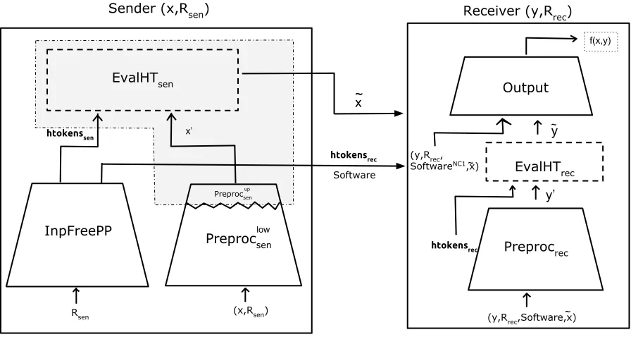
SplitState protocols. Consider the protocol Π in the bit-OT token model. We say that Π is a
SplitStateprotocol if the sender and the receiver algorithms inSplitStateprotocol are defined as
fol-lows. The sender in Π consists of the tuple of algorithms (Π.InpFreePP, Π.Preprocsen, Π.EvalHTsen). It takes as inputx with randomness Rsen and executes the following steps.
- It first executes Π.InpFreePP on input Rsen to obtain the tokens (htokenssen, htokensrec) and
Software.
- It then executes Π.EvalHTsen on input (x0,htokenssen). The procedure Π.EvalHTsen evaluates the ith token in htokens
sen with the ith bit of x0 to obtain ˜xi. The value ˜x is basically the
concatenation of all ˜xi.
- The sender then outputs (htokensrec,Software,x˜).
Notice that the third step in the above sender’s procedure involves the sender evaluating the tokens htokenssen. This seems to be an unnecessary step since the sender himself generates the tokens. Later we will see that modeling the sender this way simplifies our presentation of the proof significantly.
The receiver, on the other hand, consists of the algorithms (Π.Preprocrec, Π.EvalHTrec, Π.Output). It takes as inputy, randomnessRrec along with (htokensrec,Software, ˜x) which it receives from the sender and does the following.
- It executes Π.Preprocrec on input (y, Rrec,Software,x˜) to obtain (q,state).
- It then executes Π.EvalHTrec by querying the tokens htokensrec on input q to obtain ˜y. The
ith token inhtokensrec is queried by theith bit ofq to obtain theith bit of ˜y.
- Finally, Π.Outputis run on input (state,y˜) to obtainz which is output by the receiver.
This completes the description of Π. The following lemma shows that there exists a SplitState
protocol for a functionality if the functionality has a non-adaptive protocol.
Lemma 5. Suppose a functionality f has a non-interactive and a non-adaptive protocol in the bit-OT token model. Then, there exists a SplitState protocol for the functionality f.
Proof. Consider a non-adaptive protocol Π for a functionality f in the hardware token model. Without loss of generality, assume that it can be expressed as follows. The sender algorithm of Π, on input (x, Rsen), executes Π.GenSwTok to obtain (sware,htokens), where the length of sware is lS and the number of tokens is lT. It then sends (sware,htokens) across to the receiver. The
receiver consists of (Π.Preprocess,Π.Evaluate,Π.Output). It executes Π.Preprocess on input sware
along with its inputy and randomnessRrec to obtain queryq. It then executesEvaluateon inputq to obtain ans. Finally, Π.Output runs on inputansalong with (y, Rrec,sware) to obtain the output of the functionality. For simplicity we modify Π.GenSwToksuch that instead of outputtinghtokens
it outputs the string contained in htokens which is defined to be the concatenation of all the bits contained inhtokens.
We construct a SplitState protocol Π0 for f from Π. The sender of Π0 consists of a tuple of algorithms (Π0.InpFreePP,Π0.Preprocsen,Π0.EvalHTsen) which are defined as follows.
- Π0.InpFreePP: On input Rsen, it executes as follows. It first constructs three types of tokens described below.
– It constructs lS tokens with each token containing 0 and 1 in the first and the second
positions respectively. Recall thatlS is the size of the software output by Π.GenSwTok.
Denote this set of tokens by htokens(1)sen.
– It then chooses 2lT random bitsr1, . . . , r2lT from Rsen. Recall that lT is the number of tokens output by Π.GenSwTok. It generates 2lT tokens are generated with theith token
– It then constructs a set of lT tokens with the first token containing (r1, r2), the second
containing (r3, r4) and so on. Denote this set of tokens by htokensrec.
The output of this algorithm is (htokens(1)sen,htokens(2)sen,htokensrec). Note that this algorithm does not output any software.
- Π0.Preprocsen: On input (x, Rsen) it executes as follows. The Π0.Preprocsen first executes Π.GenSwTok(x, Rsen) to obtain (sware, s), where s is the string contained in htokens. The output of Π0.Preprocsen is (sware, s).
- Π0.EvalHTsen: On input ((sware, s),htokens(1)sen,htokens(2)sen), it does the following. It queries
htokens(1)sen on input swareto obtain ˜z1. It then queries htokens(2)sen on input sto obtain ˜z2.
The sender on input x and randomness Rsen first executes Π0.InpFreePP on input (x, Rsen) to obtain (htokens(1)sen,htokens(2)sen,htokensrec). It then executes Π0.Preprocsen on input (x, Rsen) to obtain (sware, s). Finaly Π0.EvalHTis executed on input ((sware, s),htokens(1)sen,htokens(2)sen) to obtain ˜x1 and
˜
x2. The sender sends to the receiver (˜z1,z˜2) as the software andhtokensrec as the hardware. The receiver of Π0 more or less behaves the same way as the receiver of Π. The receiver of Π0 on input (y, Rrec) and upon receiving (Software,htokens) from the sender, does the following.
- ParseSoftware as (˜z1,z˜2).
- It runs Π.Preprocesson input (y, Rrec,z˜1) to obtain q.
- Query the tokenshtokens on inputq to obtainans. Computeansg such that thei
th bit of
g
ans
is the XOR of theith bit ofansand theith bit of ˜z2.
- It then executes Π.Output on inputansg to obtain the output of the functionality.
The proof of security of Π0 can be more or less argued directly from the proof of security of Π. The main idea is that the simulator instead of giving the answersans(as in the case of Π), first outputs a random stringR as part of software. When the receiver submits its query it computesans, using the simulator of Π, and then outputs ansg , where the ith bit ofansg isansi⊕Ri, whereansi is the
ith bit ofans. The rest of the details of the simulator of Π0 is the same as the simulator of Π.
Whenever we say that a functionality has a protocol in the bit-OT token model we assume that it
is a SplitState protocol. In the class of SplitState protocols, we further consider a special class of
protocols which we term as simplified protocols.
Simplified protocols. These areSplitStateprotocols which have a trivial preprocessing algorithm on the sender’s as well as receiver’s inputs. In more detail, a protocol is said to be a simplified protocol if it is aSplitStateprotocol, and the sender’s preprocessing algorithmPreprocsen as well as the receiver’s preprocessing algorithm Preprocrec can be implemented by depth-0 circuits. Recall that depth-0 circuits which solely consists of wires and no gates. We now explore the relation between the simplified protocols and decomposable randomized encodings. We show, for every functionality, the equivalence of DRE and simplified protocols in the bit-OT token model.
Proof. Consider a functionf that takes as input of the form (x, y) whose total length is m, where
xis of lengthmxand yis of lengthmy. Suppose there exists a decomposable randomized encoding
forf, we construct a simplified protocol for f as follows. Let DRE for f consists of the following algorihtms (RE.Encode,RE.ChooseInpWires,RE.Decode). The sender of the simplified protocol, on input (x, Rsen), executes the following algorithms in order.
• InpFreePP: On input randomnessRsenit first executesRE.Encodeon input (x, Rsen) to obtain
˜
f andstate. Suppose thatstate= ((s01, s11), . . . ,(s0m, s1m)). As a simplification, we assume that all sb
i’s are bits. The argument can be extended whensbi are strings. It composes the tokens
as follows. The ith token contains the pair of bits (s0i, s1i). Denote these tokens as htokens. The tokenshtokens can be further split into sender’s tokens and receiver’s tokens. The first
mx tokens ofhtokensis denoted byhtokenssen(sender’s tokens) and the rest of the my tokens
is denoted byhtokensrec (receiver’s tokens). InpFreePP outputs ( ˜f ,htokenssen,htokensrec).
• Preprocsen: On inputx and randomnessRsen it outputsx.
• EvalHTsen: On inputx from Preprocsen and htokenssen it does the following. It evaluates the
ithtoken inhtokenssen using theith bit ofx. Let ˜xbe a concatenation of all the answers from the tokens. The output of this step is ˜x.
The output of the sender is (Software= ( ˜f ,x˜),htokensrec). We now proceed to describe the receiver. The receiver on input (y, Rrec) along with (Software= ( ˜f ,x˜),htokensrec) which it receives from the sender, it does the following. It first executesPreprocrecwhich on input (y, Rrec) outputsy. It then executes EvalHTrec which evaluates the ith token of htokensrec on input the ith bit of y to obtain the ith bit of ˜y. The receiver then executes the Output algorithm which is described as follows. It takes as input (˜y, Rrec,f ,˜x˜) and executesRE.Decode( ˜f ,x,˜ y˜) to obtainz which is output by the receiver. Firstly, it can be seen that this is a simplified protocol. Further, the correctness and privacy properties of DRE respectively implies correctness and the security of the protocol.
We now prove the other direction. Suppose there exists a simplified protocol forf then we show that there exists a decomposable randomized encoding, denoted byRE= (Encode,ChooseInpWires,
Decode), for f as follows. We first make modifications to the simplified protocol that makes the
presentation of RE easier. The InpFreePP procedure is modified such that instead of outputting the tokenshtokenssen and htokensrec, outputs the string contained in them. We further use the fact
that Preprocsen and Preprocrec are depth-0 circuits to modify them such that Preprocsen, on input
(x, Rsen), outputsxandPreprocsenon input (y, Rrec) outputsy. We now describe theREprocedure.
TheRE.Encodeprocedure takes as inputf (here we don’t distinguish between a functionality and
the circuit implementing it) and then executesInpFreePP(f, Rsen) to obtain ˜f and state(recall that
InpFreePPis modified such that it outputs the string contained in the tokens instead of outputting
the tokens.). That is, the (2i−1)th as well as the 2ith bits in the string state are precisely the
bits contained in the ith token (Again, we are making a simplification here. This argument can be generalised if (2i−1)th as well as the 2ith positions in state contains strings and not bits.). Further, the RE.Decodealgorithm takes as input ˜f along with ˜x as well as ˜y and then it executes
the Decode algorithm (of the receiver). The output of RE.Decodeis essentially the output of the
Decodealgorithm of the receiver. It follows from the security of the simplified protocol that RE is
a valid decomposable randomized encoding (and hence, a randomized encoding).
Corollary 7. There exists a simplified protocol for all functions inNC1.
4.5 Main Theorem
We now state the following theorem that shows that every function that has a non-adaptive protocol in the bit-OT token model also has a simplified protocol. Essentially this theorem says the following. Let there be a non-adaptive protocol in the bit-OT token model for a function. Then, no matter how complex the preprocessing algorithm is in this protocol, we can transform this into another protocol which has a trivial preprocessing on its inputs. Since a function having a non-adaptive protocol also has a SplitState protocol from 5, we will instead consider SplitState protocols in the below theorem.
Theorem 8. Suppose there exists a SplitState protocol for f in the bit-OT token model having
O(p(k))number of tokens, for some polynomial p. Then, there exists a simplified protocol forf in the bit-OT token model having O(p(k))number of tokens.
Proof. Consider the set S of all SplitState protocols forf each having O(p(k)) number of tokens. In this set S, consider the protocol Π0sen having the least depth complexity of Preprocsen. That is, protocol Π0sen is such that the following quantity is satisfied.
Depth(Π0sen.Preprocsen) =min Π∈S
n
Depth(Π.Preprocsen) o
We claim that the Π0sen.Preprocsen is a depth-0 circuit. If it is not a depth-0 circuit, then we arrive at a contradiction. We transform Π0sen into Π00sen, and show that Depth(Π0sen.Preprocsen) < Depth(Π00sen.Preprocsen). This would contradict the fact that the depth of Π0sen.Preprocsen is the least among all the protocols in S. To acheive the transformation, we first break Π0sen.Preprocsen
into two circuits Π0sen.Preprocupsen and Π0sen.Preproclowsen such that, Π0sen.Preprocsen will first execute Π0sen.Preproclowsen and its output is fed into Π0sen.Preprocupsen whose output determines the output of Π0sen.Preprocsen. Further, Π0sen.Preprocupsen consists of a single layer of the circuit and hence has depth 1 (If Π0sen.Preprocsen was just one layer to begin with then Π0sen.Preproclowsen would be a depth-0 circuit.). Then we define a functionality which executes the algorithms Π0sen.Preprocupsen
and Π0sen.EvalHTsen. We observe that this functionality can be realized by an NC1 circuit. Then, we proceed to replace the procedures Π0sen.EvalHTsen and Π0sen.Preprocupsen by the sender algorithm of a simplified protocol defined for this functionality, the existence of which follows from Corollary7. The Preprocsen of the resulting protocol just consists of Π0sen.Preproclowsen and this would contradict the choice of Π0sen. We now proceed to the technical details.
The sender algorithm of Π0sen can be written as (Π0sen.InpFreePP, Π0sen.Preprocsen, Π0sen.EvalHTsen) and the receiver of Π0sen can be written as (Π0sen.Preprocrec, Π0sen.EvalHTrec, Π0sen.Output). The de-scription of these algorithms are given in Section4. Consider the following functionality, denoted by fNC1.
fNCsen1(s,tempx;⊥):- On input (s,tempx) from the sender, it first executes Π0sen.Preprocupsen(tempx) to obtain x0. It then parses s as ((s01, s11), . . . ,(s0m, s1m)), where the size ofx0 is m. It then computes ˜
x= (sx 0
1
1 , . . . , s
x0m
m ), wherex0i is theith bit of x0. Finally, output ˜x. This functionality does not take
Sender (x,Rsen) Receiver (y,R rec)
EvalHTsen
InpFreePP
Preprocsen
EvalHTrec
Output
Preprocrec
Rsen (x,Rsen)
x’ htokenssen
htokensrec
Software x ~
(y,Rrec,Software,x) ~ y’
~
y
f(x,y)
htokensrec
low
Preprocsenup
(y,Rrec, SoftwareNC1,x)~
Figure 1: This represents the protocol Π0sen and the shaded area denotes the functionality fsen NC1.
Observe that fsen
NC1 is a NC
1 circuit and has a simplified protocol from Corollary 7. Let us call
this protocol ΠsenNC1. Since, the receiver’s input is⊥, the sender algorithm in this protocol does not output any tokens3. We use Π0senand ΠsenNC1 to obtain Π
00
sen. The protocol Π00senis described as follows.
Before we describe the sender algorithm of Π00sen, we modify the sender of Π0sen such that, the algorithm Π0sen.InpFreePP instead of outputting htokensrec he just outputs s, which is nothing but the string contained in htokenssen. The sender algorithm of Π00sen on input (x, Rsen), does the following.
• It first executes Π0sen.InpFreePP(Rsen) to obtain (Software, s,htokensrec), wheres, as described before is the string obtained by concatenating all the bits in htokenssen.
• It then executes Πsen.Preproclowsen on input (x, Rsen) to obtain tempx.
• It then executes the sender algorithm of Πsen
NC1 with input (s,tempx). Let the output of this algorithm be SoftwareNC1.
• Send (Software,SoftwareNC1,htokensrec) across to the receiver (recall that the sender of ΠsenNC1
does not output any tokens.).
The receiver on input (y, Rrec) along with (Software,SoftwareNC
1
,htokensrec) which it receives from the sender, does the following.
• It executes the receiver algorithm of ΠsenNC1 on input SoftwareNC 1
as well as its internal ran-domness to obtain ˜x. Note that the receiver of ΠsenNC1 does not have its own input.
• It then executes the receiver algorithm of Π0sen on input (y, Rrec,Software,x,˜ htokensrec). Let the output of this algorithm beout.
• Outputout.
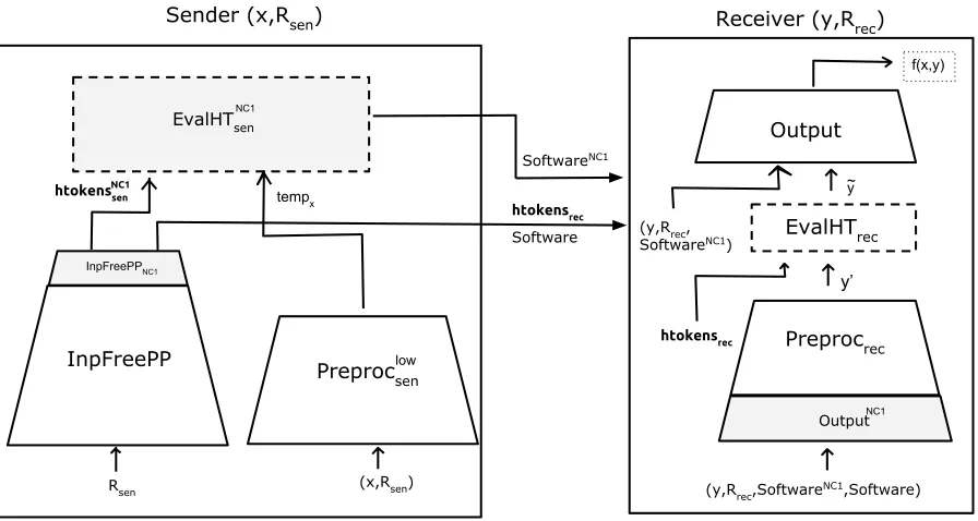
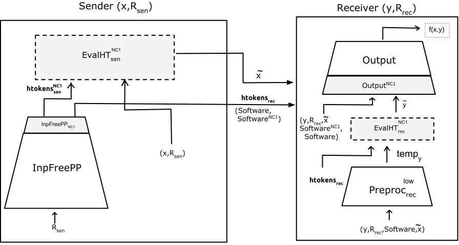
We show, in Figure 2, how we replace EvalHTsen and Preprocsenup in Π0sen by the protocol ΠsenNC1 to obtain the protocol Π00sen. We give the final decription of Π00sen in Figure3where we expand out the sender and the receiver algorithms of ΠsenNC1.
Sender (x,Rsen) Receiver (y,R
rec)
sender of
InpFreePP
EvalHTrec
Output
Preprocrec
Rsen (x,Rsen)
tempx s
htokensrec
Software
y’ ~ y
f(x,y)
htokensrec
low
sen
NC1
receiver of NC1 sen SoftwareNC1
(y,Rrec, SoftwareNC1)
string contained in htokenssen
(y,Rrec, Software)
~ x
Preprocsen
SoftwareNC1
Figure 2: In this figure, the shaded area in Figure1is replaced by the protocol ΠsenNC1.
We first claim that the protocol Π00sen satisfies the correctness property. This follows directly from the correctness of the protocols Π0sen and ΠsenNC1. The security of the above protocol is proved in the following lemma.
Lemma 9. Assuming that the protocol Π0sen andΠsenNC1 is secure, the protocolΠ00sen is secure.
Proof Sketch. To prove this, we need to construct a simulator SimΠ00
sen, such that the output of
the simulator is indistinguishable from the output of the sender of Π00sen. To do this we use the simulators of the protocols Π0sen and ΠsenNC1 which are denoted by SimΠ0
sen and SimΠsenNC1 respectively. The simulator SimΠ00
sen on input out, which is the output of the functionality f, along with
y0 which is the query made by the receiver to the OT tokens does the following. It first exe-cutes SimΠ0
sen(out, y
0) to obtain (Software,x,˜ y˜). Then, Sim
Πsen
NC1 on input ˜x is executed to obtain
SoftwareNC1. The output ofSimΠ00
sen is (Software,Software
Sender (x,Rsen) Receiver (y,R rec)
EvalHTsen
InpFreePP
Preprocsen
EvalHTrec
Output
Preprocrec
Rsen (x,Rsen)
temp
x
htokenssen
htokensrec
Software
(y,Rrec,SoftwareNC1,Software)
y’ ~ y
f(x,y)
htokensrec
low
SoftwareNC1 NC1
InpFreePPNC1
NC1
OutputNC1 (y,Rrec,
SoftwareNC1)
Figure 3: This figure depicts the protocol Π00sen after expanding out the procedures in the sender and the receiver algorithms of ΠsenNC1. The algorithmsInpFreePPNC1,EvalHT
NC1
sen (which are shaded) are part of the sender of ΠsenNC1. Since, ΠsenNC1 is a simplified protocol, its Preprocsen of ΠsenNC1 is a
depth-0 circuit. Further, the procedureOutputNC1 (shaded) is part of the receiver of ΠsenNC1. Since the sender of the protocol ΠsenNC1 does not output any tokens the receiver of ΠsenNC1 consists of just the algorithm OutputNC1.
can be shown that the output of the simulator SimΠ00
sen is indistinguishable from the output of the
sender of Π00sen.
The above lemma proves that Π00sen is a secure protocol forf. We claim that the number of tokens in Π00sen is O(p(k)). This follows directly from the fact that the number of tokens output by the sender of Π0sen is the same as the number of tokens output by Π00sen. And hence, the number of tokens output by the sender of Π00sen is O(p(k)). Further, the the depth of Preprocsen of Π00sen is strictly smaller than the depth of Π0sen.Preprocsen. This contradicts the choice of Π0sen and so, the
Preprocsen algorithm of Π0sen is a depth-0 circuit.
Now, consider a set of protocols,S0 ⊂S such that thePreprocsenalgorithms of all the protocols in S0 are implementable by depth-0 circuits. From the above arguments, we know that there is at least one such protocol in this set. We claim that there exists one such protocol in S whose
Preprocrec algorithm is implementable by a depth-0 circuit. The argument for this is similar to
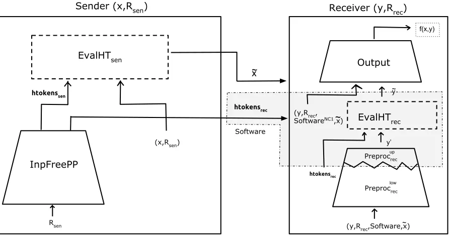
the argument for the previous case. Hence, we will highlight only those places where the argu-ment changes. Consider a protocol in S0, denoted by Π0rec such that the depth of Π0rec.Preprocrec
which contradicts the choice of Π0rec. The transformation is as follows. We split Π0rec.Preprocrecinto Π0rec.Preprocuprec and Π0rec.Preproclowrec. Also, Π0rec.Preprocuprec consists of a single layer of gates. Now consider the following functionality.
frec
NC1(str;tempy): On input (str;tempy), where str is the sender’s input and tempy is the receiver’s input, executePreprocuprecon inputtempyto obtainy0. Then, parsestras ((str10,str11), . . . ,(str0l,str1l)),
wherel denotes the length ofy0. Let ˜y be (stry 0
1
1 , . . . ,str
y0l
l ), wherey
0
i is the ith bit ofy0. Output ˜y.
Sender (x,Rsen) Receiver (y,Rrec)
EvalHTsen
InpFreePP
EvalHTrec
Output
Preprocrec
Rsen
(x,Rsen)
htokenssen
htokensrec
Software x ~
(y,Rrec,Software,x)~
y’ ~ y
f(x,y)
htokensrec
Preprocrec
low up (y,Rrec,
SoftwareNC1,x)~
Figure 4: This represents the protocol Π0rec and the shaded area denotes the functionalityfNCrec1.
Since, fNCrec1 is a NC
1 circuit, from Corollary 7 there exists a simplified protocol for frec
NC1, denoted by Πrec
NC1. We use Π 0
recand ΠrecNC1 to obtain Π00rec. The protocol Π00rec is described as follows.
Before we describe the sender of Π00rec, we modify the sender of Π0rec such that the Π0rec.InpFreePP, instead of outputtinghtokensrecoutputs a stringswhich is the concatenation of the bits inhtokensrec. The sender algorithm of Π00rec on input (x, Rsen), does the following.
• It first executes Π0rec.InpFreePP(Rsen) to obtain (Software,htokenssen, s).
• It then executes Π0rec.Preprocsen(Rsen) (which is a depth-0 circuit) on input (x, Rsen) to obtain
x0.
• It then executes Π0rec.EvalHTsen on input htokenssen and x0 to obtain ˜x.
• It then executes the sender algorithm of ΠrecNC1 with inputs. Let the output of this algorithm