A data-driven model for valve stiction

Full text

(1)To be appeared in ADCHEM 2003, Jan. 11-14, 2004, Hong Kong. A DATA-DRIVEN MODEL FOR VALVE STICTION M. A. A. Shoukat Choudhury ∗ Nina. F. Thornhill ∗∗ Sirish L. Shah ∗,1 ∗. Department of Chemical and Materials Engineering University of Alberta, Edmonton AB, Canada, T6G 2G6 ∗∗ Department of Electronic and Electrical Engineering University College London, UK, WC1E 7JE. Abstract: The presence of nonlinearities, e.g., stiction, hysteresis and backlash in a control valve limits the control loop performance. Stiction is the most common problem in spring-diaphragm type valves, which are widely used in the process industry. Though there have been many attempts (EnTech, 1998; Gerry and Ruel, 2001; Horch and Isaksson, 1998; Taha et al., 1996; Piipponen, 1996; McMillan, 1995) to understand the stiction phenomena and model it, there is lack of a proper model which can be understood and related directly to the practical situation as observed in a real valve in the process industry. This study focuses on the understanding, from real life data, of the mechanism that causes stiction and proposes a new data-driven model of stiction, which can be directly related to real valves. It compares simulation results generated using the proposed model with industrial data. Keywords: stiction, stickband, deadband, hysteresis, backlash, control valve, static friction, viscous friction, nonlinearity, slip jump, control loop performance. 1. INTRODUCTION A typical chemical plant has hundreds or thousands of control loops. Control performance is very important to ensure tight product quality and low cost of the product in such plants. The presence of oscillation in a control loop increases the variability of the process variables thus causing inferior quality products, larger rejection rates, increased energy consumption, and reduced profitability. Bialkowski (1992) reported that about 30% of the loops are oscillatory due to control valve problems. The only moving part in a control loop is the control valve. If the control valve contains static nonlinearities, e.g., stiction, backlash, and deadband, the valve output may be oscillatory which in turn can cause oscillations in the process output. Among the many types of 1. author to whom all correspondence should be addressed. E-mail: [email protected]. nonlinearities in control valves, stiction is the most common and one of the long-standing problems in the process industry. It hinders the achievement of good performance of a control valve and the control loop. Many studies (Horch, 2000; McMillan, 1995; Horch and Isaksson, 1998; Horch et al., 2000; Aubrun et al., 1995; Wallén, 1997; Taha et al., 1996; Ruel, 2000; Gerry and Ruel, 2001) have been carried out to define and detect on static friction or stiction. There is a lack of a unique definition and description of the mechanism of stiction. This work attempts to address this issue and proposes a general definition of stiction. Most of the previous studies are based on some physical model of valve friction. However, parameters of the physical model, e.g., mass of the moving parts of the valve, spring constants and forces, are not explicitly known. These parameters need to be tuned properly to produce the desired response of the valve. The effect of the change in these parameters are also not known. Working.

(2) with such a physical model is often time consuming and cumbersome for simulation purposes. Stiction and other related problems are identified in terms of the % of the valve travel or span of the valve input signal. The relationship between the magnitudes of the parameters of a physical model and deadband or backlash or stiction (expressed as a % of the span of the input signal) is not simple. The purpose of this paper is to develop an empirical data-driven model of stiction that is useful for simulation and diagnosis.. 2. WHAT IS STICTION? Different studies or organizations have defined stiction in different ways. Some of the existing definitions of stiction are reproduced below: • According to the Instrument Society of America (ISA)(ANSI/ISA-S51.1-1979) , “stiction is the resistance to the start of motion, usually measured as the difference between the driving values required to overcome static friction upscale and downscale”. The definition was first proposed in 1963 in American National Standard C85.1-1963. Though the people in the process industry do not measure stiction in this way (Ruel, 2000), this definition has not been updated till today. • According to Entech (1998), “stiction is a tendency to stick-slip due to high static friction. The phenomenon causes a limited resolution of the resulting control valve motion. ISA terminology has not settled on a suitable term yet. Stick-slip is the tendency of a control valve to stick while at rest, and to suddenly slip after force has been applied”. • According to (Horch, 2000), “The control valve is stuck in a certain position due to high static friction. The (integrating) controller then increases the set point to the valve until the static friction can be overcome. Then the valve breaks off and moves to a new position (slip phase) where it sticks again. The new position is usually on the other side of the desired set point such that the process starts in the opposite direction again”. This is an extreme case of stiction. On the contrary, once the valve overcomes stiction, it might travel smoothly for some time and then stick again when the velocity of the valve is close to zero. • In a recent paper (Ruel, 2000) reported that “stiction as a combination of the words stick and friction, created to emphasize the difference between static and dynamic friction. Stiction exists when the static (starting) friction exceeds the dynamic (moving) friction inside the valve. Stiction describes the valve’s. stem (or shaft) sticking when small changes are attempted”. This definition of stiction is close to the stiction as measured online by putting the people in process industries the loop in manual and then increasing the valve input in little increments until there is a noticeable change in the process variable. • In (Olsson, 1996), stiction is defined as “short for static friction as opposed to dynamic friction. It describes the friction force at rest. Static friction counteracts external forces below a certain level and thus keeps an object from moving”. The above discussion reveals the lack of a formal definition of stiction and the mechanism(s) that cause it. and definition of stiction. All of the above definitions agree that stiction is the static friction that keeps an object from moving and when the external force overcomes the static friction the object starts moving. But they disagree in the way it is measured and how it can be modelled. Also, there is a lack of clear description of what happens at the moment when the valve just overcomes the static friction. Some modelling approaches described this phenomena using a Stribeck effect model (Olsson, 1996). These issues can be resolved by a careful observation and a proper definition of stiction. From a detailed investigation of real process data it is observed that the phase plot of the valve input-output behavior of a valve “suffering from stiction” can be described as shown in figure 1. It consists of four components: deadband, stickband, slip jump and the moving phase. When the valve comes to a rest or changes the direction (point A in figure 1), the valve sticks. After the controller output overcomes the deadband (AB) plus the stickband (BC) of the valve, the valve jumps to a new position (point D) and continues to move. The deadband and stickband represent the behavior of the valve when it is not moving though the input to the valve keeps changing. Slip jump represents the abrupt release of potential energy stored in the actuator chamber due to high static friction in the form of kinetic energy, as the valve starts to move. The magnitude of the slip jump is very crucial in determining the limit cyclic behavior introduced by stiction (McMillan, 1995; Piipponen, 1996). Once the valve moves, it continues to move until it sticks again (point E in figure 1. In this moving phase, dynamic friction which may be much lower than the static friction is present. This section has proposed a detailed description of the effects of friction in a control valve and the mechanism and definition of stiction. The definition is exploited in the next and subsequent sections for the evaluation of practical examples and for modelling of valve stiction in a feedback control configuration..

(3) gp. ha. se. G. 1.5 1 0.5 0 -0.5 -1 -1.5 0. D B. 100. mv and op. valve input (controller output) Fig. 1. Typical input-output characteristic of a sticky valve. 1.5 1 0.5 0 -0.5 -1 -1.5. A. A. 0. 100. A. 1. 1 0 -1. 200. -1. 0. 1. controller output, op. 3. pv and op. 2. 1. 0. -1. -2 0. 200. 400 600 sampling instants. 1.5 1 0.5 0 -0.5 -1 -1.5. process output, pv. • Loop 1 is a level control loop which controls the level of condensate in the outlet of a turbine by manipulating the flow rate of the liquid condensate. Figure 2 shows the time domain data. The left panel shows time trends for condensate flow rate (pv), the controller output (op) and valve position (mv). The plots in the right panel show the characteristic plots pv-op and mv-op. The bottom figures clearly show both the deadband plus stickband and the slip jump phenomena. The slip jump is large and visible from the bottom figures especially when the valve is moving in a downscale direction. It is marked as “A” in the figure. It is evident from this figure that the valve output (mv) can never reach the valve input (op). This kind of stiction is termed as the undershoot case of valve stiction in this paper. The pv-op plot does not show the jump behavior clearly. The slip jump is very difficult to observe in the pv − op plot because process dynamics (i.e., the transfer between mv and pv) destroys the pattern. This loop shows one of the possible cases of stiction phenomena clearly. The stiction model developed here based on the control signal (op) is able to imitate this kind of behavior.. 0. Fig. 2. solid line with solid circle is pv and mv, dotted line with empty circles is op. pv and op. The objective of this section is to observe effects of stiction from the investigation of industrial control loops data. The observations reinforce the need for a rigorous definition of the effects of stiction. This section analyzes two data sets. The first data set is from a power plant and the second is from a petroleum refinery. To preserve the confidentiality of the data sources, all data are scaled and reported as mean-centered with unit variance.. -1 -1. sampling instants. 3. PRACTICAL EXAMPLES OF VALVE STICTION. 0. controller output, op. C. deadband stickband. 1. 200. sampling instants. slip jump. valve position, mv. A. process output, pv. pv and op. E. F. mo vin. valve output (process input). stickband + deadband. 0. 100. 200. 300. sampling instants. 400. 800. 1000. 1 0 -1. -1. 0. 1. controller output, op. Fig. 3. time trend of pv (solid line with solid circles) and op (dotted line with empty circles) in the top plot, closure look of the time trend (bottom left), and the pv-op plot (bottom right). • Loop 2 is a slave flow loop cascaded with a master level control loop. Time trend (Figure 3) shows clearly the undershoot case of stiction. It also shows that the valve has the slip jump phase when it overcomes stiction. Once again this slip jump is not so visible in the characteristic pv-op plot of the closed loop data (right panel of the bottom plot in figure 3), but the presence of deadband plus stickband is obvious in the plot..

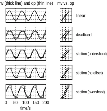
(4) 4. DATA DRIVEN MODEL OF VALVE STICTION. op(k) Look up table. A data driven model is useful because the parameters are easy to choose and the effect of these parameter change is simple to understand. The proposed data driven model has parameters that can be directly determined from plant data. The model needs only an input signal and the specification of deadband plus stickband and slip jump parameters.. (Converts mA to valve %). x(k) xss=xss y(k)=0. x(k)>0. no. yes xss=xss y(k)=100. x(k)<100. no. v_new=[x(k)-x(k-1)]/∆ ∆t xss=x(k) y(k)=y(k). sign (v_new)=sign(v_old) no. Valve sticks. yes. sticks. 4.1 Model Formulation According to most industrial personnel, the valve might be sticking only when it is at rest or it is changing its direction. When the valve changes its direction it comes to rest momentarily. Once the valve overcomes stiction, it starts moving and may keep on moving for sometime depending on how much stiction is present in the valve. At this moving phase, it suffers only dynamic friction which is much smaller than the static friction. It continues to do so until its velocity is again very close to zero or it changes its direction. In the process industries stiction is generally measured as a % of the valve travel or the span of the control signal (Gerry and Ruel, 2001). For example, a 2 % stiction means that when the valve gets stuck it will start moving only after the cumulative change of its control signal is greater than or equal to 2%. If the range of the control signal is 4 to 20 mA then 2% stiction means that a change of the control signal less than 0.32 mA in magnitude will not be able to move the valve. It measures only the deadband plus stickband. There is no information about the slip jump. To make the model parameters easily understandable by the process people, in our modelling approach the control signal has been translated to the percentage of valve travel with the help of a linear look-up table. The model consists of two parameters namely deadband plus stickband, s and slip jump, j. Figure 4 summarizes the model algorithm. • First, the controller output (mA) is provided to the look-up table where it is converted to valve travel %. • If this is less then 0 or more than 100, the valve is saturated. • If the signal is within 0 to 100% range, it calculates the slope of the controller output signal. • Then, the change of the direction of the slope of the input signal is taken into consideration. If the sign of the slope changes or remains zero for two consecutive instants, the valve is assumed to be stuck and does not move.. yes. xss=xss y(k)=y(k) no. |x(k)-xss|>s yes y(k)=x(k) - sign(v_new)*(s-j)/2. y(k) Valve characteristics (e.g., linear, square root, etc.). Valve slips and moves. (Converts valve % to mA). mv(k). Fig. 4. Flow chart for algorithm of data-driven stiction model • When the cumulative change of the input signal is more than the amount of the stickband (say, “s”), the valve slips and starts moving. • Finally, the output is again converted back to a mA signal using a look-up table based on the valve characteristics. The parameter, j signifies the slip jump start of the control valve immediately after it overcomes the deadband plus stickband. It accounts for the offset between the valve input and output signals. Different cases of stiction behavior shown in figure 5 depend on the magnitude of j.. 4.2 Open loop response of the model under a sinusoidal input Figure 5 shows the open loop behavior of the new data-driven stiction model in presence of various types of stiction. Plots in the left panel show the time trend of the valve input (thin solid line) and the output (thick solid line). The right panel shows the input-output behavior of the valve on a X-Y plot. • The first row shows the case of a linear valve without stiction. • The second row corresponds to the pure deadband without any slip jump, i.e., j = 0. Note that for this case, the magnitude of stickband is zero. • The third row shows the undershoot case of a sticky valve where j < s. This case is illustrated in the first and second examples of industrial control loops. In this case the.

(5) Table 1: Transfer function, controller and parameters for closed loop simulation. mv (thick line) and op (thin line) mv vs. op linear. deadband. stiction (undershoot). Loop type. controller pure Stiction Transfer deadband (undershoot) function Kc τI (s) s j s j. −10 s Concentration 3 e 0.2 10 10 s + 1 1 0.4 2 Level s. Stiction Stiction (no offset) (overshoot) s j s j. 5. 0. 5. 2. 5 5. 5 7. 3. 0. 3. 1.5. 3 3. 3 4.5. stiction (no offset). stiction (overshoot). 0. 50 100 150 200 time/s. Fig. 5. Open loop simulation results of the datadriven stiction model valve output can never reach the valve input. There is always some offset. • If j = s, the fourth row represents pure stickslip behavior. There is no offset between the input and output. Once the valve overcomes stiction, valve output tracks the valve input accurately. • If j > s, the valve output overshoots the desired set position or the valve input due to excessive stiction. This is termed as overshoot case of stiction. In reality a composite of these stiction phenomena may be observed. Although this model is not directly based on the dynamics of the valve, the strength of the model is that it is very simple to use for the purpose of simulation and can quantify stiction as a percentage of valve travel or span of input signal. Also, the parameters used in this model are easy to understand, realize and relate them to the real life stiction behavior. In future if it becomes possible to find some measure for quantifying stiction from closed loop operating data, it will be easy to translate this measure to the amount of stiction as a % of the span of valve input signal or % valve travel by performing some simulation studies. Though this is an empirical model and not based on physics, it is observed that this model can correctly reproduce the behavior of the physics based stiction model, the results of which are not possible to include here because of space constraints. Also, various type of valve characteristics such as equal percentage, square-root, etc. can easily be incorporated in this model (see figure 4 for further study of flow characteristic type nonlinearities.. 4.3 Closed loop behavior of the data-driven model The closed loop behavior of the stiction model has been studied in simulation. Results of two of them. are included here namely, a concentration loop and a level loop. The concentration loop has slow dynamics with large dead time. The level loop has only an integrator. The transfer functions, controllers and parameters used in simulation are shown in Table 1. Results for each case are discussed below. • Concentration loop - The transfer function model for this loop was obtained from (Horch and Isaksson, 1998). This transfer function together with the stiction model was used for closed loop simulation. Steady state results of the simulation are shown in figures 6 and 7. In both figures thin lines are the controller output. The triangular shape of the time trend of controller output is one of the characteristics of stiction (Horch, 2000). In all cases, the presence of stiction causes limit cycling of the process output. In absence of stiction there are no limit cycles, which is shown in the first row of figure 6. The presence of pure deadband also can not produce any limit cycle. It only adds dead time to the process. This conforms with the findings of (Piipponen, 1996; McMillan, 1995), where they clearly stated that the presence of pure deadband or backlash only adds dead time to the process and the presence of deadband with an integrator produces limit cycle. Figure 6 shows the controller output (op) and valve position (mv). Mapping of mv vs. op clearly shows the stiction phenomena in the valve. But it is not so evident from the mapping of pv vs. op (see figure 7). This mapping only shows some kind of elliptical loops with sharp turn around points. Therefore, if the valve position data is available one should plot valve position (mv) against the controller output (op) instead of pv versus op. • Level control loop - The closed loop simulation of the stiction model using only an integrator as the process was performed to investigate the behavior of a typical level loop in presence of valve stiction. Results are shown in figure 8. The second row of the figure shows that the deadband can produce oscillations. Again, it is observed that if there is an integrator in the process dynamics, then.

(6) mv (thick line) and op (thin line). mv vs. op linear. model. It is recommended that when using a XY plot to analyze valve problems one should use mv-op plot instead of pv-op.. pure deadband. stiction (undershoot). stiction (no offset). stiction (overshoot) 0. 100. 200. 300. time/s. Fig. 6. Closed loop simulation results of concentration loop, mv and op pv (thick line) and op (thin line). pv vs. op linear. pure deadband. stiction (undershoot). stiction (no offset). stiction (overshoot) 0. 100. 200. 300. time/s. Fig. 7. Closed loop simulation results of concentration loop, pv and op pv (thick line) and op (thin line). pv vs. op linear. pure deadband. stiction (undershoot). stiction (no offset). stiction (overshoot) 0. 100. 300 time/s. 500. Fig. 8. Closed loop simulation results of level loop, pv and op even a pure deadband can produce limit cycles, otherwise the cycle decays to zero. The pv-op plots show same kind of elliptical loops with sharp turn around.. 5. CONCLUSION A generalized definition of valve stiction based on the investigation of the real plant data have been proposed. Since the physics-based model of stiction is difficult to use because of the requirement of knowledge of mass and forces, a simple yet powerful data-driven empirical stiction model has been developed. Both closed and open loop results have been presented to show the capability of the. 6. REFERENCES Aubrun, C., M. Robert and T. Cecchin (1995). Fault detection in control loops. Control Engineering Practice 3, 1441–1446. Bialkowski, W. L. (1992). Dreams vs. reality: A view from both sides of the gap. In: Control Systems. Whistler, BC, Canada. pp. 283–294. EnTech (1998). EnTech Control Valve Dynamic Specification (version 3.0). Gerry, John and Michel Ruel (2001). How to measure and combat valve stiction online. Instrumetnation, Systems and Automated Society. Houston, Texas, USA. http://www. expertune.com/articles/isa2001/StictionMR.htm. Horch, A., A. J. Isaksson and K. Forsman (2000). Diagnosis and characterization of oscillations in process control loops. In: Proceedings of the Control Systems 2000. Victoria, Canada. pp. 161–165. Horch, A. and A. J. Isaksson (1998). A method for detection of stiction in control valves. In: Proceedings of the IFAC workshop on On line Fault Detection and Supervision in the Chemical Process Industry. Session 4B. Lyon, France. Horch, Alexander (2000). Condition Monitoring of Control Loops. PhD thesis. Royal Institute of Technology. Stockholm, Sweden. ISA Committee SP51 (1979). Process instrumentation terminology. Technical Report ANSI/ISA-S51.1-1979. Instrument Society of America. McMillan, G. K. (1995). Improve control valve response. Chemical Engineering Progress: Measurement and Control pp. 77–84. Olsson, H. (1996). Friction in control valves. PhD thesis. Lund Institute of Technology. Sweden. Piipponen, Juha (1996). Controlling processes with nonideal valves: Tuning of loops and selection of valves. In: Control Systems. Chateau, Halifax, Nova Scotia, Canada. pp. 179–186. Ruel, Michel (2000). Stiction: The hidden menace. Control Magazine. http://www.expertune .com/articles/RuelNov2000/stiction.html. Taha, Othman, Guy A. Dumont and Michael S. Davies (1996). Detection and diagnosis of oscillations in control loops. In: Proceedings of the 35th conference on Decision and Control. Kobe, Japan. Wallén, Anders (1997). Valve diagnostics and automatic tuning. In: Proceedings of the American Control Conference. Albuquerque, New Mexico. pp. 2930–2934..

(7)

No results found