Rainfall Variability, Drought Characterization, and Efficacy of Rainfall Data Reconstruction: Case of Eastern Kenya

(1)

Research Article

Rainfall Variability, Drought Characterization, and Efficacy of

Rainfall Data Reconstruction: Case of Eastern Kenya

M. Oscar Kisaka,

1

M. Mucheru-Muna,

1

F. K. Ngetich,

2

J. N. Mugwe,

2

D. Mugendi,

3

and F. Mairura

4

1_{Department of Environmental Science, Kenyatta University, P.O. Box 43844-00100, Nairobi, Kenya}

2_{Department of Agricultural Resource Management, Kenyatta University, P.O. Box 43844-00100, Nairobi, Kenya}

3_{Embu University College, P.O. Box 6-60100, Embu, Kenya}

4_{TSBF-CIAT, Tropical Soil Biology and Fertility Institute of CIAT, P.O. Box 30677-00100, Nairobi, Kenya}

Correspondence should be addressed to M. Oscar Kisaka; [email protected] Received 11 April 2014; Revised 10 August 2014; Accepted 16 August 2014

Academic Editor: Fredrick Semazzi

Copyright © M. Oscar Kisaka et al. This is an open access article distributed under the Creative Commons Attribution License, which permits unrestricted use, distribution, and reproduction in any medium, provided the original work is properly cited. This study examined the extent of seasonal rainfall variability, drought occurrence, and the efficacy of interpolation techniques in eastern Kenya. Analyses of rainfall variability utilized rainfall anomaly index, coefficients of variance, and probability analyses. Spline, Kriging, and inverse distance weighting interpolation techniques were assessed using daily rainfall data and digital elevation model using ArcGIS. Validation of these interpolation methods was evaluated by comparing the modelled/generated rainfall values and the observed daily rainfall data using root mean square errors and mean absolute errors statistics. Results showed 90% chance of below cropping threshold rainfall (500 mm) exceeding 258.1 mm during short rains in Embu for one year return period. Rainfall variability was found to be high in seasonal amounts (CV = 0.56, 0.47, and 0.59) and in number of rainy days (CV = 0.88, 0.49, and 0.53) in Machang’a, Kiritiri, and Kindaruma, respectively. Monthly rainfall variability was found to be equally high during April and November (CV = 0.48, 0.49, and 0.76) with high probabilities (0.67) of droughts exceeding 15 days in Machang’a and Kindaruma. Dry-spell probabilities within growing months were high, (91%, 93%, 81%, and 60%) in Kiambere, Kindaruma, Machang’a, and Embu, respectively. Kriging interpolation method emerged as the most appropriate geostatistical interpolation technique suitable for spatial rainfall maps generation for the study region.

1. Introduction

Understanding spatiotemporal rainfall patterns has been directly implicated to combating extreme poverty and hunger through agricultural enhancement and natural resource management [1]. The amount of soil-water available to crops depends on rainfall onset, length, and cessation which influence the success/failure of a cropping season [2]. It thus emerges that, understanding climatic parameters, rain-fall in particular, can aid in developing optimal strattegies of improving the socioeconomic well-being of smallholder farmers. This is particularly important in sub-Saharan Africa (SSA) where agricultural productivity is principally rain-fed yet highly variable [3]. Drier parts of Kenya’s central

highlands, eastern Kenya, continue to experience high unpre-dictable rainfall patterns, persistent dry-spells/droughts cou-pled with high evapotranspiration (2000–2300 mm year−1) [4]. Generally, the total amount of rainwater is enough; however, it has been reported to be poorly redistributed over time [5] with 25% of the annual rain often falling within a couple of rainstorms; as a result crops suffer from water stress, often leading to complete crop failure [6]. Recha et al. [7] noted that most studies do not provide information on the much-needed character of within-season variability despite its critical influence on soil-water distribution and productivity.

(2)

rainfall amount, rainy days, lengths of growing seasons, and dry-spell frequencies (e.g., [2,8]). Studies by Sivakumar [9], Seleshi and Zanke [10], and Tilahun [11] noted high variations in annual and seasonal rainfall totals and rainy days in Ethiopia and Sudano-Sahelian regions. Studies on rainfall patterns in the region have been based principally on annual averages, thus missing on within-season rainfall character-istics [12]. However, understanding the average amount of rain per rainy day and the mean duration between successive rain events aids in understanding long-term variability and patterns [13]. Nonetheless, meteorological stations in the region which are sole sources of climatic data are only limited to single locations spatially. In sub-Saharan Africa, the predominant setbacks in analysing hydrometeorological events are occasioned by lacking, inadequate, or inconsistent meteorological data. Like in most other places, the rainfall data within in the drier parts of Embu county and the neighbouring stations are scarce with missing data making their utilization quite intricate.

Geographic information systems (GIS) and modeling have become critical tools in agricultural research and natural resource management (NRM) yet their utilization in the study area is quite minimal and inadequate. Utilization of GIS spatial-interpolation techniques such as inverse distance weighted (IDW), Spline, and Kriging interpolation tech-niques are some of the ArcGIS application tools essential for data reconstruction. To aid in understanding spatiotemporal occurrence and patterns agro-climatic variables (e.g., rainfall) and accurate and inexpensive quantitative approaches such as GIS modelling and availabil-ity of long-term data are essential. Most meteorological data in the study area are inconsistent, unrecorded, or missing, leading to more dis-crete and unreliable data for analysis besides the main stations themselves being several kilometres from the target area. This calls for use of data reconstruction through interpolation.

On the other hand, the much-needed information on inter-/intraseasonal variability of rainfall in the region is still inadequate despite its critical implication on soil-water distribution, water use efficiency (WUE), nutrient use effi-ciency (NUE), and final crop yield. To optimize agricultural productivity in the region, there was need to quantify rainfall variability at a local and seasonal level as a first step of combating extreme effects of persistent dry-spells/droughts and crop failure. Since rainfall which is heterogeneous, in particular, is the most critical factor determining rain-fed agriculture, knowledge of its statistical properties derived from long-term observation could be utilized in developing optimal mitigation strategies in the area. To redress problems of inadequate, missing, and inconsistent point data espe-cially for ungauged areas within the study area, this study sought to further evaluate the efficacy of geostatistical and/or deterministic interpolation techniques in daily rainfall data reconstruction.

2. Materials and Methods

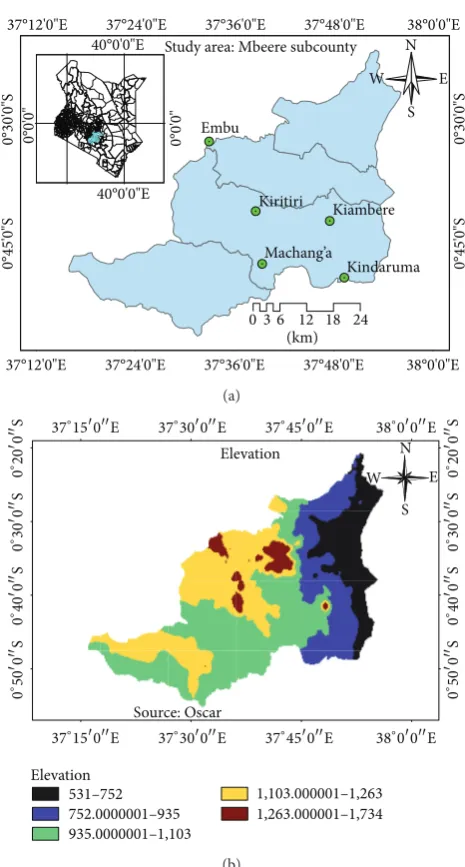
2.1. The Study Area. The study was carried out in Embu county, eastern Kenya. The rainfall data were from five rain-fall stations: Machang’a, Kiritiri, Kiambere, and Kindaruma

Embu Machang’a Kiambere Kiritiri Kindaruma N W S E 38°0'0"E 38°0'0"E 37°48'0"E 37°48'0"E 37°36'0"E 37°36'0"E 37°24'0"E 37°24'0"E 37°12'0"E 37°12'0"E 0°30'0"S 0°30'0"S 0°45'0"S 0°45'0"S 40°0'0"E 40°0'0"E 0°0'0" 0°0'0"

Study area: Mbeere subcounty

036 12 18 24 (km) (a) Elevation Elevation E N S W

531–752 752.0000001–935 935.0000001–1,103

1,103.000001–1,263 1,263.000001–1,734 Source: Oscar 0 ∘20 󳰀0 󳰀󳰀S 0 ∘30 󳰀0 󳰀󳰀S 0 ∘40 󳰀0 󳰀󳰀S 0 ∘50 󳰀0 󳰀󳰀S 0 ∘ 20 󳰀 0 󳰀󳰀 S 0 ∘ 30 󳰀 0 󳰀󳰀 S 0 ∘ 40 󳰀 0 󳰀󳰀 S 0 ∘ 50 󳰀 0 󳰀󳰀 S 37∘15󳰀0󳰀󳰀E 37∘30󳰀0󳰀󳰀E 37∘45󳰀0󳰀󳰀E 38∘0󳰀0󳰀󳰀E

37∘15󳰀0󳰀󳰀E 37∘30󳰀0󳰀󳰀E 37∘45󳰀0󳰀󳰀E 38∘0󳰀0󳰀󳰀E

(b)

Figure 1: Map showing the study area and its elevation with studied point gauged rainfall data; Machang’a and Embu, Kiritiri, Kindaruma, and Kiambere.

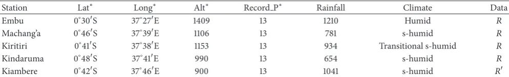
(herein commonly referred to as Mbeere region) and Embu (Embu). This region lies in the lower midlands 3, 4, and 5 (LM 3, LM 4, and LM 5), upper midlands 1, 2, 3, and 4 (UM 1, UM 2, UM 3, and UM 4), and inner lowland 5 (IL 5) [14] at an altitude of approximately 500 m to 1800 m above sea level (a.s.l) (Figure 1).

(3)

Table 1: Selected metadata of the meteorological stations used in the study.

Station Lat∗ Long∗ Alt∗ Record P∗ Rainfall Climate Data

Embu 0∘30󸀠S 37∘27󸀠E 1409 13 1210 Humid 𝑅

Machang’a 0∘46󸀠S 37∘39󸀠E 1106 13 781 s-humid 𝑅

Kiritiri 0∘41󸀠S 37∘38󸀠E 1153 13 934 Transitional s-humid 𝑅

Kindaruma 0∘48󸀠S 37∘41󸀠E 990 13 654 s-humid 𝑅

Kiambere 0∘42󸀠S 37∘46󸀠E 900 13 1041 s-humid 𝑅󸀠

∗_{Lat: latitude; Long: longitude; Alt: altitude; Record P: period of record.}

annual rainfall of less than 600 mm [14]. However, Mbeere subcounty continues to experience population pressure occa-sioned by the influx of immigrants from the overpopulated high potential areas. These areas represent Kenya’s central highlands and those of East Africa, predominant of small-holder rain-fed, nonmechanized agriculture and diminutive use of external inputs. Generally, the rainfall is bimodal with long rains (LR) from March to May and short rains (SR) from mid-October to December, hence two potential cropping seasons per year. Various agricultural studies have been carried out in the region hence the rationale behind its selec-tion. According to [15], the region has experienced drastic declines in its productivity potential rendering most farmers poor. The prime cropping activity is maize intercropped with beans though livestock keeping is equally dominant. Mbeere subcounty represents a subhumid climate region, with annual average rainfall of 781 mm while Embu is more humid with annual average rainfall above 1,210 mm (Table 1).

This region is a strategic production region, producing about 20% of the country’s maize cover. The inherently fertile Nitosols are the reasons for high-potential productivity while lower and erratic rainfall, less fertile, shallow, and sandy Ferralsols, and high drought frequency explain predominant crop failures [14]. Daily rainfall data were sourced from both the Kenya Meteorology Department and research sites with primary recording stations within the study area. The choice of rainfall stations used depended on availability of the station, the agroecological zones, and the percentage of missing data (less than 10% for a given year as required by the world meteorological organization (WMO). Much of the primary data was acquired from the ongoing recordings at Embu, Machang’a, Kiritiri, Kindaruma, and Kiambere rainfall stations.

2.2. Data Analyses. Daily primary and secondary rainfall time series were captured into MS Excel spread-sheet where seasonal rainfall totals for both Short Rains (SR) and Long Rains (LR) that is, March-April-May (MAM) and October-November-December (OND), respectively—annual average and number of rainy days were computed. In cases of high data gaps (unrecorded or missing), multiple imputations were utilized to fill in missing daily data through creation of several copies of datasets with different possible estimates. This method was preferred to single imputation and regression imputation as it appropriately adjusted the standard error for missing data yielding complete data sets for analysis [16]. Being a season-based analysis, the cumulative impact of rain-fall amount was underpinned. A rainy day was considered

to be any day that received more than 0.2 mm of rainfall as reported by the WMO. Daily rainfall data were captured into the RAINBOW software [17] for homogeneity testing based on cumulative deviations from the mean to check whether numerical values came from the same population. The cumulative deviations were then rescaled by dividing the initial and last values of the standard deviation by the sample standard deviation values:

𝑆_𝑘=∑𝑘

𝑖=1

(𝑋_𝑖− 𝑋) when𝑘 = 1, . . . , 𝑛, (1)

where 𝑆_𝑘 is the rescaled cumulative deviation (RCD), 𝑛 represents the period of record for𝑘 = 1 and also when

𝑘 = 14.

The maximum (𝑄) and the range (𝑅) of the rescaled cumulative deviations from the mean were evaluated based on number of Nil values, non-Nil values, and mean and standard deviations as well as K-S values ((2) to test homo-geneity. Low values of𝑄and𝑅would indicate that data was homogeneous:

𝑄 =max[𝑆𝑘

𝑆] ,

𝑅 =max[𝑆𝑘

𝑆] −min[

𝑆_𝑘

𝑆] ,

(2)

where𝑄is maximum (max) of𝑆_𝑘and𝑅in the range of𝑆_𝑘and Min is Minimum.

The frequency analyses were based on lognormal proba-bility distribution with log₁₀transformation using cumulative distribution function (CDF) for both LR and SR rainfall amounts. The Weibull method was used to estimate proba-bilities while the maximum likelihood method (MOM) was utilized as a parameter estimation statistic. Homogeneous seasonal rainfall totals for both seasons were then subjected to trend and variability analyses based on rainfall anomaly index (RAI) as described in [11].

Seasonal variability was computed in tandem with annual averages for both positive (3) and negative (4) anomalies using RAI;

RAI= +3 ( RF− 𝑀RF

𝑀_𝐻10− 𝑀RF

) , (3)

RAI= −3 ( RF− 𝑀RF

𝑀_𝐿10− 𝑀RF

(4)

where𝑀RFis mean of the total length of record,𝑀𝐻10is mean

of 10 highest values of rainfall of the period of record, and

𝑀_𝐿10is the lowest 10 values of rainfall of the period of record. The coefficient of variance (coefficient of variation) statis-tics were utilized to test the level of mean variations in LR and SR seasonal rainfall, number of rainy days (RD) and rainfall amounts (RA), and𝑡-test statistic to evaluate the significance of variation.

A dry day was taken as a day that received either less than 0.2 mm or no rainfall at all. A dry-spell was considered as sequence of dry days bracketed by wet days on both sides [18]. The method for frequency analysis of dry-spells was adapted from Belachew [19] as follows: in the 𝑌 years of records, the number of times(𝑖)that a dry-spell of duration

(𝑡) days occurs was counted on a monthly basis. Then the number of times(𝐼)that a dry-spell of duration longer than or equal to𝑡occurs was computed through accumulation. The consecutive dry days (1d, 2d, 3d, . . .) were prepared from historical data. The probabilities of occurrence of consecutive dry days were estimated by taking into account the number of days in a given month𝑛. The total possible number of days,

𝑁, for that month over the analysis period was computed as

𝑁 = 𝑛 ∗ 𝑌. Subsequently the probability𝑝that a dry-spell

may be equal to or longer than𝑡days was given by (5). The probability𝑞that a dry-spell not longer than𝑡does not occur at a certain day in a growing season was computed by (6); probability𝑄that a dry-spell longer than𝑡days will occur in a growing season was calculated by (7) and probability𝑝that a dry-spell exceeding𝑡days would occur within a growing season was computed by (8) as shown in the following:

𝑃 = 𝐼

𝑁, (5)

𝑞 = (1 − 𝑝) = [1 − 1

𝑁] , (6)

𝑄 = [1 − 1

𝑁]

𝑛

, (7)

𝑝 = (1 − 𝑄) = 1 − [1 −_𝑁1]𝑛. (8)

ArcGIS software tool combined with the digital elevation model (DEM) to generate average spatial rainfall and maps using various interpolation techniques was utilized for data reconstruction purposes. The stepwise methodology is sum-marized inFigure 2.

The efficacy of interpolation techniques was assessed using mean absolute errors (MAE) (9) and root mean square errors (RMSE) (10) statistics plus validation using gauged rainfall data:

MEA= 1

𝑛 𝑛 ∑ 𝑖=1

(𝑃_𝑖− 𝑂_𝑖) , (9)

RMSE= √1

𝑛 𝑛 ∑ 𝑖=1

(𝑃_𝑖− 𝑂_𝑖)2, (10)

where𝑃_𝑖and𝑂_𝑖are the predicted and observed or measured rainfall values. The𝑃− and 𝑂− are the respective means of these values and𝑛is the number of observations.

3. Results and Discussion

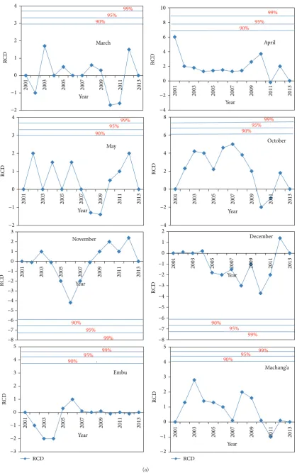
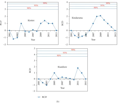
3.1. Homogeneity Testing. Homogeneity analyses had no Nil-values (Nil-values below threshold) but 100% non-Nil Nil-values (above threshold) showing high homogeneity. The standard deviations (SD) of the normalized means for both LR and SR rainfall amounts were low, for example, lowest SD = 0.1 (in Embu and Kiritiri during SRs), and highest SD = 0.9 (in Embu and Kindaruma) during LRs. Low SD values indicated the restriction of variations (rescaled cumulative deviations, RCD) around mean rainfall amounts thus high homogeneity (Table 2).

The Kolmogorov-Smirnov (K-S value) Test values, 𝑅 -Square for the seasonal rainfall, and the values of the average rainfallmeansfor rainfall months are summarized in Tables 3(a) and3(b).

A plot of homogeneity of the average monthly rainfall daily and for all stations studied showed deviations from the zero mark of the RCDs not crossing probability lines; thus homogeneity was accepted at 99% probabilities (Figure 3).

There was a normal distribution of the sampled-temporal rainfall data with high goodness-of-fit (𝑅2 = 92% to 96%) of the selected distribution showing continuity of the data from mother primary data thus high homogeneity [17]. Kolmogorov-Smirnov values (one-sided sample K-S test) showed K-S values (0.15 to 0.23) consistently lower than the K-S table value (0.302) for𝑛 = 14at𝛼 = 0.005probability indicating that an exponential, continuous distribution of the studied datasets was statistically acceptable, based on the empirical cumulative distribution function (ECDF) derived from the largest vertical difference between the extracted (observed K-S value) and the table value [20–22]. Frequency analyses of meteorological data require that the time series be homogenous in order to gain in-depth and representative understanding of the trends over time [17]. Often, nonho-mogeneity and lack of exponential distributions between datasets indicate gradual changes in the natural environment and thus trigger variability, which corresponds to changes in agricultural production [23,24].

3.2. Probabilities of Rainfall Exceedance, Return Periods, and Amounts. Results showed that there was at least 90% chance of rainfall exceeding 141.5 mm (lowest) and 258.1 mm (highest) during LRs in Kindaruma and Embu, respectively, within a return period of about 1 year (Table 4). Nonetheless, there were observably low probabilities (10%) that rains would exceed 449.8 mm and 763.0 mm during LR seasons in Machang’a and Embu, respectively, for a 10-year return period (Table 4).

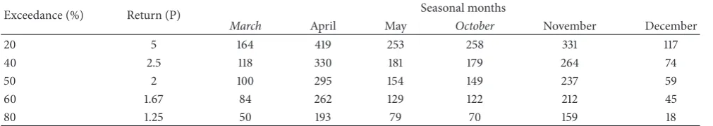
Conversely, probabilities of monthly rainfall during crop-ping seasons exceeding cropcrop-ping threshold were equally low, for example, 5% probability to exceed 419 mm in April and 331 mm in November (Table 4(b)).

(5)

Rainfall raw data

Excel processing

Best fit lines using

DEM raster ArcGIS processing

Georeferencing and extracting study area DEM raster

Map designing and cartographic cosmetic

application

Average rainfall map

Contours derivation from DEM and conversion to point

elevation

Orographic generation of rainfall data using best fit functions and

in map calculator

Spatial interpolation using various approaches and

choosing the best Rainfall data

Geo-data base (Mbeere District data from various

sources)

Boundary shapefile Generation of individual

annual rainfall layers and averaging them Rainbow software

Test of homogeneity using

Frequency analysis

Rainfall trends

altitude and rainfall amount for missing data derivation

Figure 2: Flow chart showing stepwise interpolation and data reconstruction analyses.

Table 2: Mean, standard deviation, and𝑅2values for the rainfall dailies from study stations for the period between 2001 and 2013.

Station Season Transformation Nil values Mean Standard deviation (SD) 𝑅2(%)

Embu LR log10 0 3.2 0.9 94

SR log₁₀ 0 2.7 0.1 92

Machang’a LR log10 0 2.4 0.4 96

SR log₁₀ 0 2.6 0.2 94

Kiritiri LR log10 0 2.6 0.3 94

SR log₁₀ 0 2.9 0.1 92

Kindaruma LR log10 0 2.2 0.9 88

SR log₁₀ 0 2.2 0.3 92

Kiambere LR log10 0 2.2 0.8 90

SR log₁₀ 0 2.4 0.4 96

(6)

−2 −1 0 1 2 3 4

2001 2003 2005 2007 2009 2011 2013

RC

D

Year

May

90% 95%

99%

−4 −2 0 2 4 6 8

2001 2003 2005 2007 2009 2011 2013

RC

D

Year

October

90% 95%

99%

−8 −7 −6 −5 −4 −3 −2 −1 0 1 2 3

2001 2003 2005 2007 2009 2011 2013

RC

D

Year November

99% 95% 90%

−8 −7 −6 −5 −4 −3 −2 −1 0 1 2

2001 2003 2005 2007 2009 2011 2013

RC

D

Year

December

90% 95%

99%

−4 −2 0 2 4 6 8 10

2001 2003 2005 2007 2009 2011 2013

RC

D

Year

April

90% 95%

99%

−2 −1 0 1 2 3 4

2001 2003 2005 2007 2009 2011 2013

RC

D

Year March

90% 95%

99%

−3 −2 −1 0 1 2 3 4 5

2001 2003 2005 2007 2009 2011 2013

RC

D

Year

Embu

90%

95% 99%

−2 −1 0 1 2 3 4 5

2001 2003 2005 2007 2009 2011 2013

RC

D

Year

90% 95%

99%

RCD RCD

Machang’a

(a)

(7)

−2

−1 0 1 2 3 4

2001 2003 2005 2007 2009 2011 2013

RC

D

Year Kiritiri

90% 95%

99%

−2

−1 0 1 2 3 4

2001 2003 2005 2007 2009 2011 2013

RC

D

Year Kindaruma

90% 95%

99%

−2

−1 0 1 2 3 4 5

2001 2003 2005 2007 2009 2011 2013

RC

D

Year Kiambere

90% 95%

99%

RCD

(b)

Figure 3: Rescaled cumulative deviations for seasonal months and studied rainfall stations for the period between 2000 and 2013.

Table 3: (a) Homogeneity test for the rainfall dailies from study stations for the period between 2000 and 2013. (b) Seasonal monthly (K-S value), mean, and standard deviation and𝑅2values for average rainfall dailies in both Mbeere region and Embu for the period between 2001 and 2013.

(a)

Station Season Transformation 𝑁 K-S value K-S table value

Embu LR log10 13 0.2330 0.302

∗

SR log₁₀ 13 0.1722 0.302∗

Machang’a LR log10 13 0.1479 0.302

∗

SR log₁₀ 13 0.19 0.302∗

Kiritiri LR log10 13 0.231 0.302∗

SR log₁₀ 13 0.221 0.302∗

Kindaruma LR log10 13 0.165 0.302∗

SR log₁₀ 13 0.066 0.302∗

Kiambere LR log10 13 0.127 0.302∗

SR log₁₀ 13 0.179 0.302∗

K-S: Kolmogorov-Smirnov; (K-S = 0.302∗, exponential distribution applies and is accepted). (b)

Month K-S value N Mean Standard deviation (SD) 𝑅2(%) K-S table value

Mar 0.1557 32 10.1 3.3 96 0.302∗

Apr 0.0560 32 17.2 3.9 98 0.302∗

May 0.1457 32 12.4 4.2 94 0.302∗

Jun 0.0797 32 1.3 0.3 98 0.302∗

Oct 0.0817 32 12.2 4.6 98 0.302∗

Nov 0.0961 32 15.4 3.3 98 0.302∗

Dec 0.1240 32 8.0 3.6 96 0.302∗

(8)

Table 4: (a) Probability of rainfall exceedance and return-periods for the LRs and SRs in the study area. (b) Probability of average seasonal months’ rainfall exceedance and return-periods for the LRs and SRs in Mbeere subcounty.

(a)

Exceedance (%) Return (P)

Magnitude of anticipated rainfall (mm)

Embu Machang’a Kiritiri Kindaruma Kiambere

LR SR LR SR LR SR LR SR LR SR

10 10 994.7 628.8 449.8 763 465.8 831.7 507.8 773.7 541.8 907.7

20 5 788.9 541.2 381.4 613.1 398.2 625.9 420.2 617.9 454.2 701.9

30 3.33 667.5 485.7 338.7 523.7 372.7 584.5 364.7 516.5 398.7 580.5

40 2.5 578.8 442.9 306 457.7 379.9 515.8 321.9 427.8 355.9 491.8

50 2 506.8 406.3 278.2 403.6 343.3 443.8 285.3 385.8 319.3 419.8

60 1.67 443.5 372.8 253.2 356 269.8 380.5 251.8 322.5 285.8 356.5

70 1.43 384.5 339.9 222.8 311.1 276.9 321.5 218.9 263.5 252.9 297.5

80 1.25 325.4 305.0 203.1 265.7 142 262.4 184 204.4 218 238.4

90 1.11 258.1 262.5 172.2 213.5 199.5 195.1 141.5 137.1 175.5 171.1

Exceedance (%): probability of exceedance (%) and Return (P): return period (years). (b)

Exceedance (%) Return (P) Seasonal months

March April May October November December

20 5 164 419 253 258 331 117

40 2.5 118 330 181 179 264 74

50 2 100 295 154 149 237 59

60 1.67 84 262 129 122 212 45

80 1.25 50 193 79 70 159 18

Exceedance (%): probability of exceedance (%) and Return (P): return period (years).

a successful growing season and described it as a threshold rainfall amount. During this study, the probabilities that seasonal rainfall would exceed this threshold were quite low (at most 30% for a return period of 3.33 years). Embu, being much wetter, would probably (50%) receive above threshold rainfall amount (506.8 mm) after every 2 years (Table 4). Mzezewa et al. [21] observed 47% chance of seasonal rainfall exceeding 580 mm but 0% (no increase) of exceeding total annual rainfall for a 5-year return period in the semiarid Ecotope of Limpopo, South Africa.

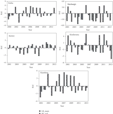
3.3. Variability and Anomalies in Seasonal Rainfall Amount. There was notable high interseasonal variability and temporal anomalies in rainfall between 2001 and 2013. Results showed neither station nor season with persistent near average (RAI = 0) rainfall especially from stations in the subhumid region. For instance, in Machang’a, the wettest LRs were recorded in 2010 (RAI = +4) while wettest SRs were recorded in 2001 (RAI = +4), 2006 (RAI = +3.8), and 2011 (RAI = +4) (Figure 4). In Embu, the highest positive anomalies (+5.0) were recorded in 2002, 2005, and 2007 during LRs (Figure 4). Noticeably, Embu appeared to be receiving more near average rainfall during SRs (2002, 2003, 2007, and 2011) contrary to the trends observed in Mbeere region (especially in Kindaruma and Kiambere) (Figure 4).

Generally, stations in subhumid areas of Mbeere sub-county recorded more negative anomalies in rainfall amount

(9)

−9

−6

−3

0 3 6 9

2000 2002 2004 2006 2008 2010 2012

RAI

Year Embu

−6.0

−3.0

0.0 3.0 6.0

2001 2003 2005 2007 2009 2011 2013

RAI

Year

−6

−3

0 3 6

2001 2003 2005 2007 2009 2011 2013

RAI

Year Kiritiri

−8

−5

−2

1 4

2001 2003 2005 2007 2009 2011 2013

RAI

Year Kindaruma

−6

−3

0 3 6

2001 2003 2005 2007 2009 2011 2013

RAI

Year Kiambere

LR_mam SR_ond

Machang’a

Figure 4: Decadal rainfall anomaly index for both LR MAM and SR OND in Embu, Machang’a, Kiritiri, Kindaruma, and Kiambere; RAI: rainfall anomaly index.

apparent that SRs recorded consistent above-average trends during this study, indicating possibilities of a reliable growing season especially for the drier Machang’a region. In tandem with this observation, findings by Hansen and Indeje (2004) and Amissah-Arthur et al. [27] observed that SRs constituted the main growing season in the drier parts of SSA and Great Horne of Africa for crops such as maize, sorghum, green grams, and finger millet.

Generally, high variability (often attributed to La Nina, El Nino, and Sea Surface Temperatures) could occasion rainfall failures leading to declines in total seasonal rainfall in the study area. According to Shisanya [25], La Nina events signif-icantly contributed to the occurrence of persistent droughts and unpredictable weather patterns during LRs in Kenya. In

contrast, El Nino events (of 1997 and 1998) have been cited as the key inputs of the positive anomalies in SR seasonal rainfall in the ASALs of Eastern Kenya [27,28].

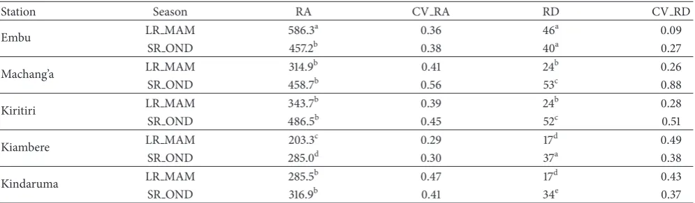
3.4. Variations in Rainfall Amounts and Number of Rainy Days. On average, the total amount of rainfall received in all stations was below 900 mm (subhumid stations) and 1400 mm (humid) per annum. Yet LRs contributed 314.9 mm and 586.3 mm while SRs contributed 438.7 mm and 479.1 mm (Table 5) translating to a total of 754 mm and 1084 mm of seasonal rainfall in in the respective station (Table 5).

(10)

Table 5: Variability analyses: coefficient of variations in seasonal rainfall amounts and number of rainy days in the study stations for the period between 2000 and 2013.

Station Season RA CV RA RD CV RD

Embu LR MAM 586.3

a _0.36 ₄₆a _0.09

SR OND 457.2b 0.38 40a 0.27

Machang’a LR MAM 314.9

b _0.41 ₂₄b _0.26

SR OND 458.7b _0.56 ₅₃c _0.88

Kiritiri LR MAM 343.7

b _0.39 ₂₄b _0.28

SR OND 486.5b 0.45 52c 0.51

Kiambere LR MAM 203.3

c _0.29 ₁₇d _0.49

SR OND 285.0d _0.30 ₃₇a _0.38

Kindaruma LR MAM 285.5

b _0.47 ₁₇d _0.43

SR OND 316.9b 0.41 34e 0.37

Values connected by the same superscript letters in the RA column denote no significant difference between the seasonal rainfall amount mean values. MAM: March-May-June and OND: October-November-December and RA: rainfall amount in (mm); RD: rainy days; CV-RA: coefficient of variation in rainfall amounts; CV-RD: coefficient of variation in rainy days.

supplied much of the total amounts of rainfall received in the region. Evaluation of variability based on coefficient of variation (CV) in rainfall amount (RA) and number of rainy days (RD) showed that most stations received highly variable rainfall.

It has been shown that a coefficient of variation (CV) greater than 30% in rainfall data series indicates massive variability in rainfall amounts and distributional patterns [29]. In Machang’a, Kiritiri, and Kindaruma, rainfall amounts during LRs were highly variable (CV = 0.41, 0.39, and 0.47, resp.) than those in Embu (CV = 0.36). Variability was equally high in the number of rainy days (RD), for example, CV = 0.51 and 0.49 in Kiritiri and Kiambere, respectively. Results also showed that LRs and SRs amounts were not significantly different from each other in most stations of Mbeere region but different in Embu (Table 5). These results indicate high variability of rainfall received across all AEZs in the study area, further evidenced by massive rainfall anomalies reported earlier by this study.

Regionally, findings of Seleshi and Zanke [10] further showed that annual and seasonal rainfall (Kiremt and Belg seasons) in Ethiopia were highly variable with CV values ranging between 0.10 and 0.50.

3.5. Monthly Variations in Seasonal Rainfall Amounts and Number of Rainy Days. Results showed that rainfall amounts received within seasonal months (March-April-May; LRs and October-November-December; SRs) were highly variable (all with CV>0.3).

Notably, coefficient of variation in Rainfall Amounts (CV-RA) was quite high during the months of March (CV-RA = 0.98) and December (RA = 0.86) in Machang’a and CV-RA = 0.61 (March) and CV-CV-RA = 0.97 (December) in Embu (Table 6). Variability in the number of rainy days (CV-RD) for each seasonal month was equally high in the two study stations. For instance, March (CV-RD = 0.61 and CV-RD = 0.47) and December (CV-RD = 0.34 and CV-RD = 83) had the highest variability in the number of rainy days in Machang’a and Embu, respectively (Table 6).

Generally, onset months (March and October) and ces-sation months (May and December) received highly variable rainfall amounts compared to mid-seasonal months. Notably, Machang’a, though being more of an arid region, generally recorded lower variability in number of rainy days during SR seasonal months compared to those recorded at Embu during the same season, evidence of reduced variability and wetting of SRs in the region. In addition, it was evident that the amount of rainfall and number of rainy days received in the past decade in most stations were more consistent (temporally) in April and November but highly unpredictable in March (onset) and December (cessation). This signifi-cantly affects the cropping calendar in rain-fed agricultural productivity of the region. Nonetheless, lower values of variations in the number of rainy days (CV-RD) indicated that variations in rainy days were fairly consistent compared to variations in rainfall amounts received. It would also appear that most stations in Mbeere region received more rainfall during SR season with November alone accounting for about 60% of total seasonal rainfall amount received while April accounts for 51% of the LR rainfall in the case of Machang’a. Conversely, Embu received more rainfall during LRs with April accounting for about 52% of total rainfall received. These trends indicate that SR seasons would be receiving more rainfall amounts than LRs in the region, a trend acknowledged by most (67.3%) smallholder farmers in SSA, Amissah-Arthur et al. [27] and Barron et al. [12]. Trends of high variability in seasonal monthly rainfall reported by this study have also been cited by Mzezewa et al. [21] who reported high coefficient of variation for seasonal (315%) and annual (50–114%) rainfall in semiarid Ecotope, northeast of South Africa. Additionally, Sivakumar [9] found that annual rainfall in the Sudano-Sahelian zone of West Africa was less variable (0.36) than monthly (0.54) rainfall.

(11)

Table 6: Variability in rainfall amounts and number of rainy days during seasonal months for studied stations for the period between 2000 and 2013.

Parameter March April May October November December

Embu

RA (mm) 110.1 300.8 175.6 175.1 250.3 71.8

CV-RA 0.61 0.48 0.54 0.66 0.43 0.97

RD 20 14 12 10 13 17

CV-RD 0.47 0.27 0.27 0.59 0.25 0.83

Machang’a

RA (mm) 85.5 160.2 69.2 98.9 267.9 72

CV-RA 0.98 0.42 0.69 0.8 0.77 0.86

RD 8 11 5 14 29 10

CV-RD 0.61 0.22 0.61 0.35 0.23 0.34

Kiritiri

RA (mm) 88.7 167.1 87.9 110.4 274.3 101.8

CV-RA 0.61 0.48 0.54 0.66 0.43 0.97

RD 7 14 3 12 24 16

CV-RD 0.47 0.27 0.27 0.59 0.25 0.83

Kiambere

RA (mm) 41.8 97.8 63.8 45 147 93

CV-RA 0.88 0.46 0.59 0.83 0.67 0.81

RD 3 12 2 11 17 9

CV-RD 0.51 0.2 0.53 0.31 0.23 0.4

Kindaruma

RA (mm) 59.5 119.5 86.5 48.6 165.6 102.6

CV-RA 0.46 0.31 0.37 0.59 0.29 0.84

RD 2 12 3 9 18 7

CV-RD 0.62 0.48 0.52 0.46 0.36 0.84

RA (mm): rainfall amount in millimetres; CV-RA: coefficient of variation in rainfall amounts, RD: number of rainy days; CV-RD: coefficient of variation in rainy days.

March (0.72 and 0.55) and December (0.8 and 0.6) in average subhumid (Machang’a, Kiritiri, Kiambere, and Kindaruma) stations and humid ones (Embu), respectively (Figure 5). The probability of having a dry-spell increased with shorter periods (for instance, more chance of having a 3-day than a 10- or 21-day dry-spell) (Figure 5).

On the other hand, the probabilities that dry-spells would exceed these day durations were equally high (Figure 6). There was 70% chance that dry-spells would exceed 15 days in average Mbeere stations and 50% in Embu (Figure 6).

Dry-spells during cropping months are quite common which often trigger reduced harvests or even complete crop failures, in the study region. Rainfall being a prime input and requirement for plant life in rain-fed agriculture, the occurrence of dry-spells has particular relevance to rain-fed agricultural productivity (Belachew, 2002; Rockstrom et al., 2002). It was observed that lowest probabilities of occurrence of dry-spells of all durations were recorded in the month of April (during LRs) and November (during SRs). The occurrence of dry-spells of all durations decreased from April towards May (LR) and November towards December (SRs). Indeed, the months of April and December coincide with the peak of rainfall amounts for both SR and LR growing

(12)

0 0.2 0.4 0.6 0.8 1 Ma r Ap r

May Oct No

v

Dec Ma

r

Ap

r

May Oct No

v

Dec Ma

r

Ap

r

May Oct No

v

Dec Ma

r

Ap

r

May Oct No

v

Dec Ma

r

Ap

r

May Oct No

v

Dec

Embu Kiritiri Kiambere Kindaruma

for n da ys Dr y-sp ell p roba b ili ty

Seasonal-cropping months per site

21days 7days 15days 5days 10days 3days Machang’a

Figure 5: Probability of a dry-spell of length≥𝑛days, for𝑛 = 3, 5, 7, 15, and 21, in each seasonal-cropping month, based on raw rainfall data from 2000 to 2013 for studied humid and subhumid stations.

Ma

r

Ap

r

May Oct No

v

Dec Ma

r

Ap

r

May Oct No

v

Dec Ma

r

Ap

r

May Oct No

v

Dec Ma

r

Ap

r

May Oct No

v

Dec Ma

r

Ap

r

May Oct No

v Dec 0 0.2 0.4 0.6 0.8 1

Embu Kiritiri Kiambere Kindaruma

P roba b ili ty o f ex cee d an ce

Seasonal rainfall months per site 21 days 15 days 10 days 7 days 5 days 3days Machang’a

Figure 6: Probability of dry-spells exceeding the𝑛 (3, 5, 7, 10, 15, and21)days for each seasonal month calculated using the raw rainfall data from 2000 to 2013 for studied humid and subhumid stations.

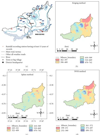
3.7. Spatial Average Rainfall Interpolations (ArcGIS Spatial Analyst Application). Performance of the different interpo-lation techniques was varied. Kriging and Spline techniques reported more representative values of observed rainfall when compared to the IDW method. Generally, Kriging spatial interpolation capability for rainfall amounts was found to be high (predicting 670–742 mm for observed 800 mm) (Figure 7). Evidently, lower eastern parts of the region received low rainfall amounts as interpolated across all the test methods (ranging from 229 to 397 mm), adequately replicating trends of the actual observed rainfall. Trends of the region receiving high rainfall at Siakago (1200 mm p.a.) were adequately predicted in Kriging and IDW when com-pared to Spline prediction (Figure 7).

Evaluation of the mean absolute error (MAE) and root mean square error (RMSE) between reconstructed interpo-lated) and observed rainfall data further showed that the Kriging method (MAE = 147 mm and RMSE = 176.5 mm)

Table 7: Mean absolute error, RMSE, and 𝑅2 values for the interpolation produced from validation of IDW, Kriging, and Spline methods.

IDW Kriging Spline

Average P (O) 371.3 (760) 507.6 (760) 399.4 (760)

SD 115.5 137.5 106.7

MAE 276.7 147.6 248.6

RMSE (mm) 294.7 176.5 264.7

𝑅2 _0.04 _0.67 _0.23

P: predicted precipitation; O: Observed precipitation; SD: standard devi-ation; MAE: mean absolute error; RMSE: root mean square error; IDW: inverse weighted mean.

would be the best-bet technique to adopt for rainfall inter-polation for the region (Table 7).

(13)

Main road, tarmac

Other all-weather roads River

Town or big village District headquarter

Rainfall recording station having at least₁₅years of records

(a)

Kriging method

0 510 20 30 40 (km)

Mbeere_boundary

362–397 398–409

410–509

510–669

670–742 N W

S E

(b)

37.23 37.39 37.55 37.71 37.87 37.23 37.39 37.55 37.71 37.87

−0.95

−0.76

−0.57

−0.38

−0.2

−0.95

−0.76

−0.57

−0.38

−0.2

(km) 0 510 20 30 40

Spline method

Mbeere_boundary

229–₃₂₁ 322–409

410–509

510–669

670–742 N W

S E

(c)

.23 .39 .55 .71 .87 0 510 20 30 40

(km)

IWM method

Mbeere_boundary

198–251 252–360

361–372

373–₄₉₇

498–551 N W

S E

(d)

Figure 7: Annual rainfall maps of observed and those of reconstructed rainfall using IWM, Kriging, and Spline interpolation techniques.

Figure 8shows the scatter plots of recorded versus pre-dicted (interpolated) decadal average rainfall across the study stations based on Kriging interpolation technique.

A comparison of the predicted and recorded rainfall amounts showed further best-fit performance of the Kriging interpolation technique in ArcGIS. Predictions in Machang’a recorded high values of best-fit (𝑅2 = 0.92) compared to Kiambere (𝑅2 = 0.64) which could be attributed to high

missing data in the raw rainfall dailies in the latter station (Figure 8).

(14)

R² = 0.7583

650 800 950 1100

650 700 750 800 850 900 950

Reco

rd

ed ra

infall (mm)

Predicted rainfall (mm) Embu

R² = 0.92

400 550 700 850 1000

500 540 580 620

Reco

rd

ed ra

infall (mm)

Predicted rainfall (mm)

Reco

rd

ed ra

infall (mm)

R² = 0.85

400 550 700 850 1000

400 500 600 700 800

Predicted rainfall (mm) Kiritiri

Reco

rd

ed ra

infall (mm)

R² = 0.64

400 550 700 850 1000

300 400 500 600

Predicted rainfall (mm) Kiambere

Reco

rd

ed ra

infall (mm)

R² = 0.81

400 550 700 850 1000

300 400 500 600

Predicted rainfall (mm) Kindaruma

Rainfall

Machang’a

Figure 8: Comparison between recorded and ArCGIS Kriging predicted average decadal rainfall amount across study stations: error bars denote standard deviation of observed means,𝑛 = 13.

On the other hand, Kriging is a geostatistical method, which is based on statistical models that include autocorrelation, which underpins the statistical relationships among the measured and predicted data points [32]. Better prediction of the Kriging method established in this study could be attributed to its capability of producing a prediction surface, thus providing a measure of the certainty or accuracy of the predictions. In this study, the resultant patterns of spatial distribution for each map were an outcome of the generated patterns from the mapping of the index value (the mean annual precipitation) and as influenced by the spatial local conditions (elevation) including the nonexistence of altitudi-nal variability of the parameters of the distribution function and the interpolation methods used. Statistically, the spatial

distribution of quantiles is theoretically better underpinned in Kriging method than in the other methods tested. For this study, Kriging was extended by the regional regression for each index value for areas whose terrain or other controls could have contributed to the spatial variability of the trends, explaining its better predictability.

4. Conclusion and Recommendations

(15)

patters. Weibull method for estimating probabilities and method of moment (MOM) parameter estimation methods proved to be sufficient for the task, in evaluating data series homogeneity and frequency. Decadal rainfall trends showed that both long rains (LRs) and average annual rainfall have decreased in the past 13 years in the region. Mbeere region appeared to have experienced pronounced declines in rainfall amounts especially those received during LRs. Nonetheless, rainfall amount during SRs markedly increased in most study stations, with high amount gains established in the Mbeere stations. Evidently, probabilities that seasonal rainfall amounts would exceed the threshold for cropping (500– 800 mm) were quite low (10%) in all stations. The amount of rainfall received during LRs and SRs varied significantly in Embu but not in Machang’a. There was evidence of increas-ing rainfall variability from Embu station towards Mbeere stations to as high as CV = 0.88 in Machang’a. Probabilities that the region would experience dry-spells exceeding 15 days during a cropping season were equally high, for example, 46% in Embu and 87% in Machang’a. This replicates high chances that soil moisture could be lost by evaporation bearing in mind the high chances (81%) that the same dry-spells exceeding 15 days could reoccur during the cropping season. On the other hand, Kriging technique was identified as the most appropriate (𝑅2 = 0.67) geostatistical interpolation techniques that can be used in spatial and temporal rainfall data reconstruction in the region. Based on these findings, it is apparent that farmers in the lower eastern Mbeere region are encouraged to intensify cropping during SRs as compared to LRs. It is equally important that they schedule supplementary irrigation, only based on timely, regular, and accurate dissemination daily monthly and seasonal forecasts by the Kenya Meteorological Department. High rainfall variability and chances of prolonged dry-spells established in this study also demand that farmers ought to keenly select crop varieties and types that are more drought resistant (sorghum and millet) other than common maize cropping. For instance, probabilities of having dry-spells exceeding 15 days are relatively high (63%, 80%, 91%, 93%, and 57% for Machang’a, Kiritiri, Kiambere, Kindaruma, and Embu, resp.) during both SR and LR seasons. In this regard, the choice of crop variety and type should be based on the degree of its tolerance to drought. These decisions can be optimized if the probability of dry-spells is computed after successful (effective) planting dates. There is need for establishing further precise, timely weather forecasting mechanisms and communication systems to guide on seasonal farming. In most arid and semiarid regions, soil moisture availability is primarily dictated by the extent and persistency of dry-spells. It is thus essential to match the crop phenology with dry-spell lengths based days after sowing to meet the crop water demands during the sensitive stages of crop growth. Knowledge of lengths of dry-spells and the probability of their occurrence can also aid in planning for supplementary risk aversion strategies through prediction of high water demand spells.

Conflict of Interests

The authors declare that there is no conflict of interests regarding the publication of this paper.

Acknowledgment

Special thanks are extended to RUFORUM fiscal support.

References

[1] IPCC, “Climate change,” Fourth Assessment Report, Cam-bridge University Press, CamCam-bridge, Mass, USA, 2007. [2] K. F. Ngetich, M. Mucheru-Muna, J. N. Mugwe, C. A. Shisanya,

J. Diels, and D. N. Mugendi, “Length of growing season, rainfall temporal distribution, onset and cessation dates in the Kenyan highlands,”Agricultural and Forest Meteorology, vol. 188, pp. 24– 32, 2014.

[3] M. R. Jury, “Economic impacts of climate variability in South Africa and development of resource prediction models,”Journal of Applied Meteorology, vol. 41, no. 1, pp. 46–55, 2002.

[4] A. N. Micheni, F. M. Kihanda, G. P. Warren, and M. E. Probert, “Testing the APSIM model with experiment data from the long term manure experiment at Machang’a (Embu), Kenya,”

inModeling Nutrient Management in Tropical Cropping Systems,

R. J. Delve and M. E. Probert, Eds., pp. 110–117, Australian Center for International Agricultural Research (ACIAR) No 114, Canberra, Australia, 2004.

[5] S. K. Kimani, S. M. Nandwa, D. N. Mugendi et al., “Principles of integrated soil fertility management,” inSoil Fertility Man-agement in Africa: A Regional Perspective, M. P. Gichuri, A. Bationo, M. A. Bekunda et al., Eds., pp. 51–72, Academy Science Publishers (ASP); Centro Internacional de Agricultura Tropical (CIAT); Tropical Soil Biology and Fertility (TSBF), Nairobi, Kenya, 2003.

[6] G. A. Meehl, T. F. Stocker, W. D. Collins et al., “Global climate projections,” in Climate Change: The Physical Science Basis, S. Solomon, D. Qin, M. Manning et al., Eds., Cambridge University Press, Cambridge, UK, 2007.

[7] C. Recha, G. Makokha, P. S. Traor´e, C. Shisanya, and A. Sako, “Determination of seasonal rainfall variability, onset and cessation in semi-arid Tharaka district, Kenya,”Theoretical and Applied Climatology, vol. 108, no. 3-4, pp. 479–494, 2011. [8] E. M. Mugalavai, E. C. Kipkorir, D. Raes, and M. S. Rao,

“Analysis of rainfall onset, cessation and length of growing season for western Kenya,”Agricultural and Forest Meteorology, vol. 148, no. 6-7, pp. 1123–1135, 2008.

[9] M. V. K. Sivakumar, “Empirical-analysis of dry spells for agricultural applications in SSA Africa,”Journal of Climate, vol. 5, pp. 532–539, 1991.

[10] Y. Seleshi and U. Zanke, “Recent changes in rainfall and rainy days in Ethiopia,”International Journal of Climatology, vol. 24, no. 8, pp. 973–983, 2004.

[11] K. Tilahun, “Analysis of rainfall climate and evapo-transpiration in arid and semi-arid regions of Ethiopia using data over the last half a century,”Journal of Arid Environments, vol. 64, no. 3, pp. 474–487, 2006.

(16)

[13] P. B. I. Akponikp`e, K. Michels, and C. L. Bielders, “Integrated nutrient management of pearl millet in the sahel using com-bined application of cattle manure, crop residues and mineral fertilizer,”Experimental Agriculture, vol. 46, pp. 333–334, 2008. [14] R. Jaetzold, H. Schmidt, Z. B. Hornet, and C. A. Shisanya,

Farm Management Handbook of Kenya, vol. 11/C ofNatural

Conditions and Farm Information, Ministry of agriculture/GTZ, Nairobi, Kenya, 2nd edition, 2007.

[15] J. Mugwe, D. Mugendi, M. Mucheru-Muna, D. Odee, and F. Mairura, “Effect of selected organic materials and inorganic fertilizer on the soil fertility of a Humic Nitisol in the central highlands of Kenya,”Soil Use and Management, vol. 25, no. 4, pp. 434–440, 2009.

[16] C. K. Enders,Applied Missing Data Analysis, The Guilford Press, New York, NY, USA, 2010.

[17] D. Raes, P. Willems, and F. Baguidi, “Rainbow:-a software package for analyzing data and testing the homogeneity of historical data sets,” in Proceedings of the 4th International Workshop on ‘Sustainable man agement of marginal dry lands’, pp. 27–31, Islamabad, Pakistan, January 2006.

[18] K. K. Kumar and T. V. R. Rao, “Dry and wet spellsat Campina Grande-PB,”Revista Brasileira de Meteorologia, vol. 20, no. 1, pp. 71–74, 2005.

[19] A. Belachew,Dry-spell Analysis for Studying the Sustainability of Rain-Fed Agriculture in Ethiopia: The Case of the Arbaminch Area, International Commission on Irrigation and Drainage (ICID), Institute for the Semi-Arid Tropics, Direction de la meteorology nationale du Niger, Addis Ababa, Ethiopia, 2000. [20] J. J. Botha, J. J. Anderson, D. C. Groenewald et al., “On-farm

application of in-field rainwater harvesting techniques on small plots in the central region of South Africa,” The Water Research Commission Report, 2007.

[21] J. Mzezewa, T. Misi, and L. Ransburg, “Characterization of Rainfall at a Semi-arid Ecotope in the Limpopo Province (South Africa) and its Implications for Sustainable Crop Production,” 2013,http://www.wrc.org.za/.

[22] MATLAB (Matrix Laboratory), “The Empirical Cumulative Distribution Function: ECDF,” 2013, http://www.mathworks .com/help/stats/ecdf.html.

[23] F. A. Huff and S. A. Changnon Jr., “Precipitation modification by major urban areas,”Bulletin of the American Meteorological Society, vol. 54, pp. 1220–1232, 1973.

[24] N. Bayazit, “A comprehensive theory of participation in plan-ning and design (P&D),”Design: Science: Method, pp. 30–47, 1981.

[25] C. A. Shisanya, “The 1983-1984 drought in Kenya,”Journal of East Africa Resource Development, vol. 20, pp. 127–148, 1990. [26] M. Hulme, “Climatic perspectives on SSA desiccation: 1973–

1998,”Global Environmental Change, vol. 11, no. 1, pp. 19–29, 2001.

[27] A. Amissah-Arthur, S. Jagtap, and C. Rosen-Zweig, “Spatio-temporal effects ofEl Ni˜noevents on rainfall and maize yield in Kenya,”International Journal of Climatology, vol. 22, no. 15, pp. 1849–1860, 2002.

[28] A. Anyamba, C. J. Tucker, and J. R. Eastman, “NDVI anomaly Pattern over Africa during the 1997/98ENSOWarm Event,” International Journal of Remote Sensing, vol. 24, pp. 2055–2067, 2001.

[29] A. Araya and L. Stroosnijder, “Assessing drought risk and irrigation need in Northern Ethiopia,”Agricultural and Forest Meteorology, vol. 151, no. 4, pp. 425–436, 2011.

[30] J. R. Kosgei,Rainwater harvesting systems and their influences on field scale soil hydraulic properties, water fluxes and crop production [Ph.D. thesis], University of KwaZulu-Natal, Pieter-maritzburg, South Africa, 2008.

[31] P. Burroughs and A. McDonald,Principles of Geographical Infor-mation Systems: Land Resources Assessment, Oxford University Press, New York, NY, USA, 1998.

(17)