ISSN 2286-4822 www.euacademic.org
Impact Factor: 3.4546 (UIF) DRJI Value: 5.9 (B+)
Weibull Distribution Modelling Using the LLSM
Approach: Application to Wind Speed Variation
SULAIMON MUTIU O.
Department of Statistics & Mathematics Moshood Abiola Polytechnic, Abeokuta, Ogun State Nigeria
SODUNKE MOBOLAJI A.
Department of Science Laboratory Technology Moshood Abiola Polytechnic, Abeokuta, Ogun State Nigeria
Abstract:
The most significant constraint of the wind force is the wind speed. Wind speed varies with the day and the season of the year and even some extent from year to year. Wind energy has inherent variances and hence it has been expressed by distribution functions. For this rationale, understanding wind ratings via Weibull distribution is very important. In this paper, We model the wind speed in Ikeja area of Lagos, Nigeria (Ikeja being the capital of Lagos, and Lagos being the most populous city of Nigeria, the second fastest-growing city in Africa and the seventh in the world) using among other methods, the Linear Least Square Method (LLSM) to estimate the Weibull distribution parameters, namely, shape parameter (k) and scale parameter (c). The Weibull distribution is an important distribution especially for reliability and maintainability analysis. The suitable values for both shape parameter and scale parameters of Weibull distribution are important for selecting locations of installing wind turbine generators. The scale parameter of Weibull distribution is also important to determine whether a wind farm is good or not.
Introduction
Navigation and agriculture have been using wind energy for centuries, but it is only during recent times that wind energy has been getting a lot of awareness due to the concentration on inexhaustible energies. The successful fitting of statistical distributions like the Weibull Distribution to wind speed data in wind energy means having a thorough understanding of the wind features at any particular location. Not only is understanding wind ratings important, but at the same time how to interpret the Weibull distributions for wind velocity is also crucial. Precise data about wind velocity is significant to determine best sites for wind turbines. Wind speeds also have to be calculated by those who are apprehensive about the dispersion of airborne pollutants.
Apart from this the energy requirement of the world is always increasing by 4-5% every year while fossil fuel reserves which address this want are decreasing much quicker than the
need. Additionally, with the increasing, depressing
consequences of fossil fuels on the environment, primarily developed countries and others have started utilizing renewable energy sources. These days, the most growing and most commonly utilized energy source is wind energy. Thus, when using energy from the wind, the most crucial parameter, that is wind velocity, has to be calculated, and this is where Weibull distributions play a part.
policy viewpoint. Among various renewable energy resources, wind power energy is one of the most popular and promising energy resources in the whole world today (Paritosh Bhattacharya, 2010).
At a specific wind farm, the available electricity generated by a wind power generation system depends on mean wind speed (MWS), standard deviation of wind speed, and the location of installation. Since year-to-year variation on annual MWS is hard to predict, wind speed variations during a year can be well characterized in terms of a probability distribution
function (Paritosh Bhattacharya, 2010). This paper in addition
addresses the relations among MWS, its standard deviation, and the two important parameters of the Weibull distribution.
Related Work
Materials and Methods
Wind Speed Data
Measured wind speed data are commonly available in time series format, in which each data point represents either an instantaneous sample wind speed or an average wind speed over some time period. An example of such data (giving yearly over a 13 year period is given) in Table 1 obtained from the Nigerian Meteorological Agency.
The Weibull Distribution of the Wind Speed
The Weibull distribution (named after the Swedish physicist Weibull, who applied it when studying material in tension and fatigue in the 1930s) provides a close approximation to the probability laws of many natural phenomena. It has been used to represent wind speed distribution for application in wind load studies for some time. In recent years most attention has been focused on this method for wind energy application not only due to its greater flexibility and simplicity but also because it can give a good fit to experimental data (Indhumathy, Seshaiah and Sukkiramathi, 2014).
Wind power developers measure actual wind resources, in part, to determine the distribution of wind speeds because of its considerable influence on wind potential. The Weibull wind speed distribution is a mathematical idealization of the distribution of wind speed over time (Odo, Offiah and Ugwuoke, 2012).
In statistical modelling of wind speed variation, the
Weibull two-parameter (shape parameter k and scale
parameter c) function have been widely used by many
researchers. The function shows the probability of the wind
speed being in a 1m/s interval centred on a particular speed (u),
The Weibull distribution is characterized by two parameters;
one is the shape parameter k (dimensionless) and the other is
the scale parameter c (m/s) with its probability density function
(pdf) defined as:
( ) . / . / [ . / ]; ---(1)
where ( ) is the probability of observing wind speed u, k is the
dimensionless Weibull shape parameter, c is the Weibull scale
parameter, which have reference values in the units of wind speed.
The corresponding cumulative distribution function (cdf)
of the Weibull distribution is given as:
( ) ∫ ( ) [ . / ] ---(2)
where ( ) is the cumulative probability function of observing
wind speed u.
In Weibull distribution, the variations in wind speed are characterized by two functions which are the probability
density function (pdf) and the cumulative distribution function
(cdf). The pdf indicates the fraction of time (or probability) for
which the wind is at a given speed u while the cdf of the speed
u gives the fraction of the time (or probability) that the wind
speed is equal or lower than u.
Estimation of Average and Standard Deviation of the Wind Speed
The average wind speed can be expressed as
̅ ∫ ( ) ∫ . / [. / ] [ . / ] ---(3)
Let . / and . /
Equation (3) can be simplified as
By substituting a Gamma Function
( ) ∫ into Equation (4) and let then
we have
̅ . / ---(5)
The standard deviation of the wind speed u is given by
√∫ ( ̅) ( ) ---(6)
That is
√∫ ( ̅ ̅ ) ( )
√∫ ( ) ̅∫ ( ) ∫ ̅ ( )
√∫ ( ) ̅ ̅ ̅
√∫ ( ) ̅ ̅ ̅
√∫ ( ) ̅ ---(7)
But ∫ ( ) ∫ . / [. / ] [ . / ] ---(8)
Using appropriate substitution and transformation as with Equation (3), we have
∫ ( ) . / ---(9)
Hence we get
√ . / 0 . /1
0 . / . /1
Computation of Weibull Parameters (k and c) of the Wind Speed
Several methods could be applied to calculate the wind speed distribution among which are Linear Least Square Mehtod (LLSM), Maximum Likelihood Method (MLM), Modified Maximum Likelihood Method (MMLM), Power Density Method (PDM), Mean Standard Deviation Method (MSDM) and Method of Moments (MOM).
In this paper we employed the Linear Least Square
Method (LLSM) in computing the Weibull parameters. Linear least square method (LLSM) is used to calculate the parameter(s) in a formula when modelling an experiment of a phenomenon and it can give an estimation of the parameters (Paritosh Bhattacharya, 2010). Linear least square method is extensively used in engineering and mathematics problems that are often not thought of as an estimation problem (Salahaddin A. Ahmed, 2013).
With the help of this method the parameters are estimated with regression line equation by cumulative density function. From Equation (2), the cumulative distribution function of the Weibull distribution with two parameters was written as:
( ) [ . / ]
This function can be arranged as:
( ) [. / ] ---(11)
If we take the natural logarithm of Equation (11)
2
( )3 [. / ] ---(12)
And then retake the natural logarithm of Equation (12), we get the following equation:
0 2
Equation (13) can be written as a linear equation as:
---(14)
where Y = 0 2
( )31 ---(15)
---(16)
---(17)
and ---(18)
By regression formula
∑ ∑ ∑
∑ (∑ ) ---(19)
∑ ∑ ∑ ∑
∑ (∑ )
---(20)
and ---(21)
The parameters k and c could equally be written in terms of the
natural logarithm as
∑ , * ( )+- ∑ ∑ , * (
∑ (∑ )
---(22)
2 ∑ ∑ , * (
3 ---(23)
There are various approaches to obtaining the empirical distribution function from that: one method is to obtain the
vertical coordinate for each point. Let be a
random sample of , ( ) is estimated and replaced by the
median rank method as follows (Y. Lei, 2008):
( )
---(24)
where is the rank of the data point and is the number of
data points.
Predicted Weibull Wind Speed (̂) Model
The predicted wind speed value ( ̂) can be obtained from
Equation (24) as
Equation (15) gives ( ̂) as
( ̂) [ ⁄ ̂] ---(26)
where ̂ is the estimated Y value from Equation (14)
Prediction Performance of the Weibull Distribution Model
The prediction accuracy of the model in the estimation of the wind speeds with respect to the actual values were evaluated based on three tests in this article, first is the coefficient of
determination R2 used to how well the regression model
describes the data, second is root mean square error (RMSE) and third is the coefficient of efficiency (COE). These tests were computed based on the following equations:
,∑ ( ̅)( ̂
̅)-,∑ ( ̅) -,∑ ( ̂ ̅) - ---(27)
0 ∑ ( ̂) 1 ---(28)
∑ ( ̂)
∑ ( ̅) ---(29)
where is the actual or measured wind speed data, ̂ is the
predicted wind speed data with the Weibull distribution, ̅ is
the mean of the actual wind speed data and is the number of
observations.
Weibull Reliability Function
The Weibull reliability function is defined as
( ) ( ) [ . / ] ---(30)
By manipulating Equation (30) for reliability, reliability is
achieved after time t as
, - ---(31)
Results Output
Table 1: Computation of Weibull Parameters (k and c) from the
Measured Wind Speed (u)
1998 1999 2000 2001 2002 2003 2004 2005 2006 2007 2008 2009 2010 Jan 4.3 4.6 6.1 6.1 6 4 5 5.9 7.2 4.4 5.6 5.8 2.8
Feb 4.9 4.3 4.2 7.1 8 5 3 8.2 8.7 8.7 6.9 8 3
Mar 5 5.6 7.8 8.7 8.6 5 3 8.5 8.4 9 9.3 8.8 3
Apr 5.2 5.6 7.6 7.6 7.6 5 5 8.6 9 9.8 8.1 9.1 3
May 4.2 4.1 6.3 6.4 6.5 3 3 7.1 6.1 6.8 6.4 7.4 3
Jun 3.9 6.8 5.9 6 6.9 3 3 6.5 5.9 7.7 5.9 5.3 3
Jul 5.1 6.1 7.1 7.7 8 3 3 8.4 8.7 9.8 5.1 6.5 3
Aug 5.9 5.2 7.3 8.7 9.7 4 3 10.3 9.7 10.5 6.7 8.2 3
Sep 5.1 7.5 6.3 7.4 2.5 4 2 8.2 8 7.6 4.8 6.1 3.3
Oct 3.8 5.6 5.8 5.7 5.9 3 2 5.4 5.5 5.7 4.2 5.1 3
Nov 3.9 3.5 5.3 5.8 5.1 3.7 2 5.5 4.1 5.9 3.9 5.7 3.1
Dec 3.7 5.1 5.8 5.9 5.5 3.5 2 5.1 5 5 3.8 5 3.1
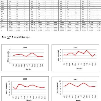
̅ 4.5833 5.3333 6.2917 6.9250 6.6917 3.8500 3.0000 7.3083 7.1917 7.5750 5.8917 6.7500 3.0250 σ 0.7056 1.1364 1.0308 1.0972 1.8985 0.8017 1.0445 1.6318 1.8168 2.0316 1.6930 1.4829 0.1138 Range 2.2 4 3.6 3 7.2 2 3 5.2 5.6 6.1 5.5 4.1 0.5 k 1.3369 1.3945 1.4629 1.6035 1.4383 1.2962 1.2777 1.6481 1.5661 1.6558 1.4800 1.5770 1.2609 c 8.6890 8.4551 8.3065 8.1283 8.1900 8.8784 8.9725 8.0213 8.0464 7.9324 8.1812 8.0983 9.1358
̅̅ ∑ ̅
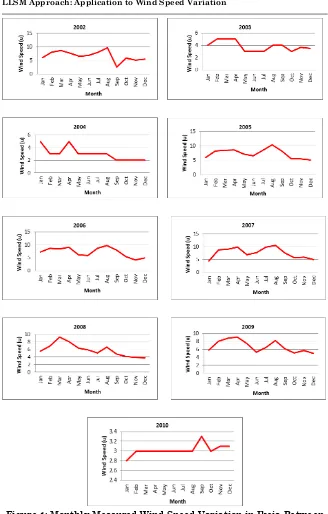
Figure 2: Yearly Measured Wind Speed Variation in Ikeja Between 1998 and 2010.
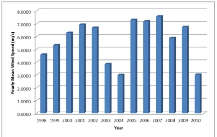
Figure 3: Yearly Mean Wind Speed Variation in Ikeja Between 1998 and 2010.
Table 2: Weibull Probability Distribution f(u) of the Measured Wind
Speed
1998 1999 2000 2001 2002 2003 2004 2005 2006 2007 2008 2009 2010
Jan 0.0822 0.0846 0.0808 0.0883 0.0809 0.0808 0.0754 0.0922 0.0789 0.0973 0.0852 0.0890 0.0809
Feb 0.0797 0.0856 0.0888 0.0813 0.0661 0.0766 0.0821 0.0739 0.0657 0.0692 0.0766 0.0725 0.0807
Mar 0.0792 0.0798 0.0687 0.0674 0.0614 0.0766 0.0821 0.0710 0.0684 0.0661 0.0574 0.0653 0.0807
Apr 0.0782 0.0798 0.0702 0.0772 0.0692 0.0766 0.0754 0.0700 0.0630 0.0580 0.0672 0.0626 0.0807
May 0.0825 0.0861 0.0795 0.0864 0.0775 0.0829 0.0821 0.0838 0.0870 0.0869 0.0802 0.0776 0.0807
Jun 0.0834 0.0724 0.0820 0.0888 0.0746 0.0829 0.0821 0.0884 0.0883 0.0790 0.0835 0.0913 0.0807
Jul 0.0787 0.0769 0.0740 0.0763 0.0661 0.0829 0.0821 0.0720 0.0657 0.0580 0.0877 0.0846 0.0807
Aug 0.0744 0.0819 0.0725 0.0674 0.0528 0.0808 0.0821 0.0534 0.0566 0.0511 0.0781 0.0707 0.0807
Sep 0.0787 0.0675 0.0795 0.0789 0.0871 0.0808 0.0810 0.0739 0.0720 0.0800 0.0889 0.0872 0.0802
Oct 0.0836 0.0798 0.0826 0.0904 0.0815 0.0829 0.0810 0.0944 0.0904 0.0942 0.0905 0.0921 0.0807
Nov 0.0834 0.0869 0.0852 0.0899 0.0860 0.0817 0.0810 0.0940 0.0938 0.0932 0.0908 0.0895 0.0806
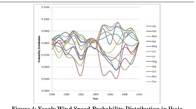
Figure 4: Yearly Wind Speed Probability Distribution in Ikeja between 1998 and 2010.
Table 3: Cumulative Probability Distribution of the Measured Wind Speed
1998 1999 2000 2001 2002 2003 2004 2005 2006 2007 2008 2009 2010
Jan 0.0822 0.0846 0.0808 0.0883 0.0809 0.0808 0.0754 0.0922 0.0789 0.0973 0.0852 0.0890 0.0809
Feb 0.1618 0.1701 0.1696 0.1695 0.1470 0.1574 0.1575 0.1660 0.1446 0.1665 0.1619 0.1615 0.1617
Mar 0.2411 0.2500 0.2383 0.2369 0.2083 0.2339 0.2396 0.2370 0.2130 0.2326 0.2193 0.2268 0.2424
Apr 0.3193 0.3298 0.3086 0.3141 0.2776 0.3105 0.3149 0.3071 0.2760 0.2906 0.2865 0.2894 0.3232
May 0.4018 0.4159 0.3881 0.4005 0.3550 0.3934 0.3970 0.3908 0.3630 0.3775 0.3667 0.3671 0.4039
Jun 0.4852 0.4883 0.4700 0.4893 0.4296 0.4763 0.4791 0.4793 0.4513 0.4565 0.4502 0.4584 0.4847
Jul 0.5639 0.5652 0.5440 0.5657 0.4957 0.5591 0.5612 0.5512 0.5170 0.5145 0.5379 0.5430 0.5654
Aug 0.6383 0.6471 0.6165 0.6330 0.5485 0.6399 0.6433 0.6046 0.5736 0.5656 0.6160 0.6137 0.6461
Sep 0.7171 0.7146 0.6960 0.7119 0.6356 0.7207 0.7243 0.6785 0.6457 0.6456 0.7050 0.7010 0.7264
Oct 0.8007 0.7944 0.7786 0.8023 0.7171 0.8035 0.8053 0.7729 0.7361 0.7398 0.7954 0.7930 0.8071
Nov 0.8841 0.8814 0.8638 0.8922 0.8031 0.8852 0.8864 0.8670 0.8299 0.8330 0.8862 0.8825 0.8877
Dec 0.9679 0.9638 0.9463 0.9816 0.8870 0.9674 0.9674 0.9623 0.9224 0.9298 0.9770 0.9749 0.9683
Table 4: Predicted Wind Speed (̂) from the Weibull Parameters (k
and c)
1998 1999 2000 2001 2002 2003 2004 2005 2006 2007 2008 2009 2010
Jan 4.3083 4.6167 6.1391 6.1031 6.1563 4.0121 4.9788 5.9136 7.3481 4.1935 5.6918 5.8314 2.7996
Feb 4.9107 4.3002 4.1242 7.1563 7.9843 4.9893 3.0104 8.3039 8.6948 8.8332 6.8079 8.0505 3.0001
Mar 5.0093 5.6379 7.7191 8.6345 8.4585 4.9893 3.0104 8.5734 8.4453 9.0848 8.9982 8.7343 3.0001
Apr 5.2045 5.6379 7.5467 7.6477 7.6487 4.9893 4.9788 8.6608 8.9342 9.7004 8.0709 8.9723 3.0001
May 4.2062 4.0873 6.3378 6.4280 6.6473 2.9947 3.0104 7.2269 6.2143 6.9866 6.5134 7.4917 3.0001
Jun 3.8976 6.7720 5.9373 5.9933 7.0244 2.9947 3.0104 6.5858 5.9969 7.9138 6.0057 5.2721 3.0001
Jul 5.1072 6.1239 7.0996 7.7429 7.9843 2.9947 3.0104 8.4848 8.6948 9.7004 5.1554 6.5854 3.0001
Aug 5.8674 5.2365 7.2812 8.6345 9.2370 4.0121 3.0104 9.9607 9.4533 10.1738 6.9998 8.2281 3.0001
Sep 5.1072 7.3791 6.3378 7.4542 2.3577 4.0121 1.9943 8.3039 8.0970 7.8153 4.8267 6.1592 3.2995
Oct 3.7940 5.6379 5.8352 5.6598 6.0557 2.9947 1.9943 5.3347 5.5535 5.7472 4.1586 5.0446 3.0001
Nov 3.8976 3.4428 5.3149 5.7716 5.2237 3.7099 1.9943 5.4516 3.9431 5.9796 3.8213 5.7208 3.1001
Dec 3.6902 5.1346 5.8352 5.8828 5.6453 3.5067 1.9943 4.9816 4.9860 4.9167 3.7088 4.9303 3.1001
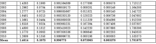
Table 5: Weibull Parameters, Model Performance Parameters and Reliability Test
Year
Weibull Parameters Model Performance
Parameters 90% Reliability
k c(m/s) R2 RMSE COE
1998 1.3369 8.6890 0.999705310 0.011690 0.000299 1.614112
1999 1.3945 8.4551 0.998222281 0.047012 0.001867 1.683752
2000 1.4629 8.3065 0.998315821 0.044694 0.002051 1.783801
2002 1.4383 8.1900 0.991594889 0.177898 0.009578 1.713112
2003 1.2962 8.8784 0.999859173 0.009281 0.000146 1.564388
2004 1.2777 8.9725 0.999885667 0.011821 0.000140 1.541722
2005 1.6481 8.0213 0.993283120 0.128223 0.006736 2.047602
2006 1.5661 8.0464 0.995980028 0.111329 0.004096 1.912288
2007 1.6558 7.9324 0.992665231 0.167394 0.007406 2.037807
2008 1.4800 8.1812 0.992419823 0.142220 0.007698 1.788398
2009 1.5770 8.0983 0.997808336 0.066640 0.002203 1.943833
2010 1.2609 9.1358 0.999996731 0.000198 0.000003 1.533373
Mean 1.4614 8.3873 0.996773 0.073965 0.003378 1.781675
Discussion of Results
In this study, wind speed data for Ikeja, Nigeria, over a 13 year period from 1998 to 2010 were analysed. The analysis were done using Microsoft Excel® package. The Weibull distribution
parameters in terms of k and c, mean wind speed, probability
distribution, cumulative probability distribution and predicted wind speed were determined.
Figure 1 shows the monthly wind speed variation in Ikeja over the period of 13 years from 1998 to 2010, while the yearly mean wind speed values, standard deviations and ranges are presented in Table 1. It can be seen in Table 1 that the highest yearly mean wind speed of 7.5750 m/s occurs in the year 2007, while the minimum mean wind speed of 3.0000m/s occurs in the year 2004. The highest yearly wind speed standard deviation of 2.03160 also occurs in the year 2007, while the minimum mean wind speed of 0.1138 occurs in the year 2010.
Table 2 shows the Weibull probability distribution of the measured wind speed, Table 3 shows the Weibull cumulative probability distribution of the measured wind speed and Table 4 shows the predicted wind speed energy from the Weibull parameters for the 13 years period.
The model prediction performance parameters (R2,
Estimated mean shape parameter (k) indicates which
implies that on the average wind energy fall rate increases yearly in Ikeja, Nigeria.
Mean value of 0.996773 for R2 indicates that
approximately 99.7% of the total variation in the wind speed energy in Ikeja area of Lagos, Nigeria is being explained by the Weibull distribution model.
The recorded low value of the wind speed mean RMSE indicates better fit of the Weibull distribution model to the measured wind speed data. This implies that the model accurately predicts the wind speed energy in Ikeja area of Lagos, Nigeria.
The Mean COE value of 0.003378 indicates that on the average wind speed energy is approximately 0.338% efficient in Ikeja area of Lagos, Nigeria.
The 90% reliability estimate indicates that wind speed energy in Ikeja area of Lagos, Nigeria will on the average be reliable for approximately 1.8years.
The results give the model equation as:
In[ –ln{1 – F(u)}] = –3.11 + 1.46lnu ---(32)
Conclusion
wind energy is on the average of approximately 20 months. If the need be to select a wind turbine for Ikeja, the most favourable cut-in speed should on the average be approximately 5.72 (m/s).
It is recommended that the analyses be extended to other locations in Nigeria where installation of wind energy conversion systems is being proposed.
REFERENCES
Indhumathy, Seshaiah, Sukkiramathi (2014). Estimation of Weibull Parameters for Wind Speed Calculation at
Kanyakumari in India. International Journal of
Innovative Research in Science, Engineering and Technology. Vol. 3, Issue 1, January 2014.
Justu C. G., Mikhilai A. (1976). Height Variation of Wind Speed
and Wind Distribution Statistics. Geophys Res Lett , Vol
3 , pp .261-4 ,1976.
Odo F. C., Offiah S. U., Ugwuoke P. E. (2012). Weibull Distribution-based Model for Prediction of Wind
Potential in Enugu, Nigeria. Adv. Appl. Sci. Res., 2012,
3(2):1202-1208.
Paritosh Bhattacharya (2010). A Study on Weibull Distribution
for Estimating The Parameters. Journal of Applied
Quantitative Methods. Vol5 No.2, summer 2010.
Y. Lei (2008). Evaluation of Three Methods for Estimating the Weibull Distribution Parameters of Chinese Pine (Pinus
tabulaeformis). Journal of Forest Science, 54, 2008 (12):
566–571.
Salahaddin A. Ahmed (2013): Comparative Study of Four Methods for Estimating Weibull Parameters For
Halabja, Iraq. International Journal of Physical Sciences
Online
http://www.brighthub.com/environment/renewable-energy/articles/107129.aspx
http://www.engineeredsoftware.com/nasa/weibull.htm https://www.en.m.wikipedia.org/wiki/Lagos