R E S E A R C H
Open Access
Dynamics of a modified Nicholson-Bailey
host-parasitoid model
Abdul Qadeer Khan
*and Muhammad Naeem Qureshi
*Correspondence:
[email protected] Department of Mathematics, University of Azad Jammu and Kashmir, Muzaffarabad, 13100, Pakistan
Abstract
In this paper, we study the qualitative behavior of the following modified Nicholson-Bailey host-parasitoid model:
xn+1= bxne–ayn
1 +dxn
, yn+1=cxn
(1 –
e–ayn),
wherea,b,c,dand the initial conditionsx0,y0are positive real numbers. More precisely, we investigate the boundedness character, existence and uniqueness of a positive equilibrium point, local asymptotic stability and global stability of the unique positive equilibrium point, and the rate of convergence of positive solutions of the system. Some numerical examples are also given to verify our theoretical results. MSC: 39A10; 40A05
Keywords: modified Nicholson-Bailey model; boundedness; local stability; global character; rate of convergence
1 Introduction
Many ecological models are governed by differential as well as difference equations. In particular, ecological models with non-overlapping populations are better formulated as discrete dynamical systems compared to the continuous time models. These models have been extensively studied in recent years because of their wide applicability to the study of population dynamics [, ]. In fact, in the case of discrete dynamical systems, one has more efficient computational results for numerical simulations and also has rich dynamics as compared to the continuous ones. In recent years, several papers have been published on the mathematical models of biology that discuss the system of difference equations generated from the associated system of differential equations as well as the associated numerical methods [, ]. In mathematical biology, the model such as the host-parasitoid has attracted many researchers during the last few decades. Usually, the biologists believe that a unique, positive, locally asymptotically stable equilibrium point in an ecological sys-tem is very important []. Therefore, it is pertinent to find conditions which may guarantee the global stability of a positive equilibrium point, if it exist, for the given system. See [] for introduction to mathematical models in biological sciences.
The prime example of an ecologically interesting discrete-time model for interacting populations is the Nicholson-Bailey model for host-parasitoid dynamics. Parasitoids are insect species whose larvae develop by feeding on the bodies of other arthropods, usually
killing them. Larvae emerge from the host and develop into free-living adults. The adults then lay their eggs in a subsequent generation of hosts. Most parasitoid larvae require a specific life-stage of the host, so parasitoid and host generations are linked to one an-other. Consequently host-parasitoid models often use a discrete time step corresponding to the common generation length of host and parasitoid. The classic model was derived by Nicholson and Bailey (). The assumptions of the Nicholson-Bailey model are as follows:
(i) Hosts are distributed at random, at densityxnper unit area in generationn.
(ii) Parasitoids search at random and independently, each having an ‘area of discovery’ a, and lay an egg in each host found.
(iii) Each parasitized host gives rise to one new parasitoid in generationn+ . (iv) Each unparasitized host gives rise tob> new hosts in generationn+ .
Each parasitoid attacks the hosts found inaunits of area, so the expected number of hosts attacked by each parasitoid isax. The expected total number of attacks isaxy. The total number of attacks can also be written as the sum over hosts of the number of attacks on each host. All hosts have the same expected number of attacks, so the expected number of attacks on any given host must beay. Under the assumptions listed above, the number of eggs per host has a Poisson distribution. Consequently, the expected fraction of hosts that are not parasitized is the probability that a Poisson random variable with meanay
takes the value zero. The resulting population dynamics are
xn+=bxne–ayn, yn+=cxn
–e–ayn.
Here,xnandynrepresent the densities of the host and parasitoid population at yearn.
bis the number of offspring of an unparasitized host surviving to the next year. Assum-ing random encounter between hosts and parasitoids, the probability that a host escapes parasitism can be approximated bye–ayn, whereais a proportionality constant. Similarly, the probability to become infected is then given by –e–ayn. The parametercdescribes the number of parasitoids that hatch from an infected host.
Now, assume that the host has bounded dynamics in absence of parasitoid,i.e., has self-regulation (density dependence). For example, assume host dynamics are inherently lo-gistic (e.g., the Beverton-Holt model).
Then a modified form of the Nicholson-Bailey host-parasitoid model is
xn+=
bxne–ayn
+dxn
, yn+=cxn
–e–ayn, ()
wherea,b,c,dand the initial conditionsx,yare positive real numbers.
Section discusses the boundedness character of the model. Section is about the exis-tence and uniqueness of the positive equilibrium point. It also contains the local stability of the equilibrium point. Section discusses the global behavior of the equilibrium point. Whereas Section is about the rate of convergence and Section gives the numerical examples of the proved results. In the last section a brief conclusion is given.
2 Linearized stability
Let us consider the two-dimensional discrete dynamical system of the form
xn+=f(xn,yn),
(v) An equilibrium point(x¯,¯y)is called an asymptotic global attractor if it is a global attractor and stable.
Definition . Let (x¯,y¯) be an equilibrium point of the mapF(x,y) = (f(x,y),g(x,y)), where
Lemma .[] Consider the second-degree polynomial equation
λ–pλ–q= , ()
where p and q are real numbers.
(i) If both roots of Equation()lie in the open unit disk|λ|< ,then the equilibrium point(x¯,y¯)is locally asymptotically stable.
(ii) If at least one of the roots of Equation()has absolute value greater than one,then the equilibrium point(x¯,¯y)is unstable.
(iii) A necessary and sufficient condition for both roots of Equation()to lie inside the open disk|λ|< is
|p|< –q< .
In this case the locally asymptotically stable equilibrium(x¯,¯y)is also called a sink. (iv) A necessary and sufficient condition for both roots of Equation()to have absolute
value greater than one is
|q|> , |p|<| –q|.
In this case(x¯,y¯)is a repeller.
(v) A necessary and sufficient condition for one root of Equation()to have absolute value greater than one and for the other to have absolute value less than one is
p+ q> , |p|>| –q|.
In this case the unstable equilibrium(x¯,¯y)is called a saddle point.
(vi) A necessary and sufficient condition for a root of Equation()to have absolute value equal to one is
|p|=| –q|.
In this case the equilibrium(x¯,y¯)is called a non-hyperbolic point.
3 Boundedness
The following theorem shows that every positive solution {(xn,yn)}∞n= of system () is bounded.
Theorem . Every positive solution{(xn,yn)}∞n=of system()is bounded.
Proof Let{(xn,xn)}∞n=be any positive solution of system (), then
xn+=
bxne–ayn
+dxn
≤bxn
dxn
≤b
d, n= , , . . . . ()
Also
yn+=cxn
–e–ayn≤cx
n≤
bc
Hence from () and (), we have
Proof It follows from induction.
4 Existence and uniqueness of a positive equilibrium point and local stability The following theorem shows the existence and uniqueness of a positive equilibrium point of system ().
(),the following statements hold true:
(i) The unique positive equilibrium point of system()is locally asymptotically stable if and only if
(ii) The unique positive equilibrium point is a repeller if and only if
abcreacr(bdr+–b( +)(bdrbdr(eacr)(bdr+–b)– ) – )
and
(iii) The unique positive equilibrium point is a saddle point if and only if
(iv) The unique positive equilibrium point is non-hyperbolic if and only if
beacr(bdr+–b)(acr( +bdr)+ )
Proof (i) The characteristic polynomial of the Jacobian matrixFJ(x¯,y¯) about the
equilib-rium point (x¯,y¯) is given by
Let
p=be
acr(bdr+–b)(acr( +bdr)+ ) ( +bdr) ,
q=ab
creacr(bdr+–b)(bdr(eacr(bdr+–b)– ) – ) ( +bdr) .
Then it follows from Lemma . that the unique positive equilibrium point (x¯,y¯) of system () is locally asymptotically stable if and only if
beacr(bdr+–b)(acr( +bdr)+ ) ( +bdr) < –
abcreacr(bdr+–b)(bdr(eacr(bdr+–b)– ) – ) ( +bdr) < .
Obviously, one can prove (ii), (iii) and (iv).
5 Global character
Lemma .[] Let I= [a,b]and J= [c,d]be real intervals,and let f :I×J→I and g:I×
J→J be continuous functions.Consider system()with initial conditions(x,y)∈I×J.
Suppose that the following statements are true:
(i) f(x,y)is non-decreasing inxand non-increasing iny. (ii) g(x,y)is non-decreasing in both arguments.
(iii) If(m,M,m,M)∈I×Jis a solution of the system
m=f(m,M), M=f(M,m),
m=g(m,m), M=g(M,M)
such thatm=Mandm=M,then there exists exactly one equilibrium point (x¯,¯y)of system()such thatlimn→∞(xn,yn) = (x¯,y¯).
Theorem . Assume that ac+d>abc,then the unique positive equilibrium point(x¯,¯y)
in[,bd]×[,bcd]of system()is a global attractor.
Proof Letf(x,y) =bxe+–dxay andg(x,y) =cx( –e–ay). Then it is easy to see thatf(x,y) is non-decreasing inxand non-increasing iny. Moreover,g(x,y) is non-decreasing in both argu-mentsxandy. Let (m,M,m,M) be a positive solution of the system
m=f(m,M), M=f(M,m),
m=g(m,m), M=g(M,M).
Then one has
m=
bme–aM +dm
, M=
bMe–am +dM
()
and
m=cm
–e–am, M =cM
From () one has from Lemma . the unique positive equilibrium point of system () is a global
Lemma . The unique positive equilibrium point(x¯,¯y)in[,bd]×[,bcd]of system()is globally asymptotically stable if and only if
beacr(bdr+–b)(acr( +bdr)+ ) ( +bdr) < –
abcreacr(bdr+–b)(bdr(eacr(bdr+–b)– ) – ) ( +bdr) < .
Proof The proof is a direct consequence of Theorems . and ..
6 The rate of convergence
In this section we will determine the rate of convergence of a solution that converges to the unique positive equilibrium point of system ().
The following result gives the rate of convergence of solutions of the system of difference equations
Xn+=
A+B(n)Xn, ()
whereXnis anm-dimensional vector,A∈Cm×mis a constant matrix, andB:Z+→Cm×m
is a matrix function satisfying
B(n) → ()
asn→ ∞, where · denotes any matrix norm which is associated with the vector norm
(x,y) =x+y.
Proposition .(Perron’s theorem []) Suppose that condition()holds.If Xnis a
so-lution of(),then either Xn= for all large n or
ρ= lim
n→∞
Xn
/n
exists and is equal to the modulus of one of the eigenvalues of matrix A.
Proposition .[] Suppose that condition()holds.If Xnis a solution of(),then
either Xn= for all large n or
ρ= lim
n→∞ Xn+
Xn
exists and is equal to the modulus of one of the eigenvalues of matrix A.
Let{(xn,yn)}be any solution of system () such thatlimn→∞xn=x¯ andlimn→∞yn=y¯.
To find the error terms, one has from system ()
xn+–x¯=
bxne–ayn
+dxn
–bxe¯ –ay¯ +dx¯
= be
–ayn ( +dxn)( +dx¯)
(xn–x¯) +
bx¯(e–ayn–e–ay¯)
( +dx¯)(yn–¯y)
and
Now the limiting system of error terms can be written as
which is similar to the linearized system of () about the equilibrium point (x¯,y¯). Using proposition (.), one has following result.
Theorem . Assume that {(xn,yn)} is a positive solution of system () such that
of every solution of()satisfies both of the following asymptotic relations:
lim
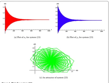
(a) Plot ofxnfor system () (b) Plot ofynfor system ()
(c) An attractor of system ()
Figure 1 Plots for system (23).
Example Leta= .,b= .,c= .,d= .. Then system () can be written as
xn+=
.xne–.yn
+ .xn
, yn+= .xn
–e–.yn, n= , , . . . , ()
with initial conditionsx= .,y= ..
In this case the unique positive equilibrium point of system () is given by (x¯,¯y) = (., .). Moreover, in Figure the plot ofxnis shown in Figure (a), the plot
ofynis shown in Figure (b) and an attractor of system () is shown in Figure (c).
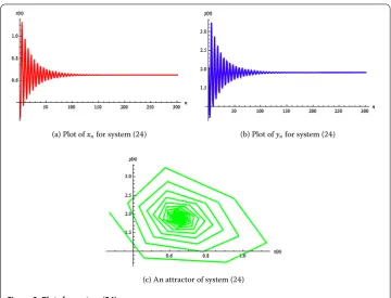
Example Leta= .,b= .,c= .,d= .. Then system () can be written as
xn+=
.xne–.yn
+ .xn
, yn+= .xn
–e–.yn, n= , , . . . , ()
(a) Plot ofxnfor system () (b) Plot ofynfor system ()
(c) An attractor of system ()
Figure 2 Plots for system (24).
In this case the unique positive equilibrium point of system () is given by (x¯,¯y) = (., .). Moreover, in Figure the plot of xn is shown in Figure (a), the
plot of yn is shown in Figure (b) and an attractor of system () is shown in
Fig-ure (c).
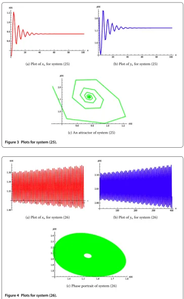
Example Leta= .,b= .,c= .,d= .. Then system () can be written as
xn+=
.xne–.yn
+ .xn
, yn+= .xn
–e–.yn, n= , , . . . , ()
with initial conditionsx= .,y= ..
In this case the unique positive equilibrium point of system () is unstable. Moreover, in Figure the plot ofxnis shown in Figure (a), the plot ofynis shown in Figure (b) and
a phase portrait of system () is shown in Figure (c).
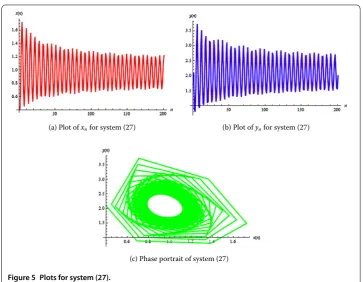
Example Leta= .,b= .,c= .,d= .. Then system () can be written as
xn+=
.xne–.yn
+ .xn
, yn+= .xn
–e–.yn, n= , , . . . , ()
with initial conditionsx= .,y= ..
In this case the unique positive equilibrium point of system () is unstable. Moreover, in Figure the plot ofxnis shown in Figure (a), the plot ofynis shown in Figure (b) and
(a) Plot ofxnfor system () (b) Plot ofynfor system ()
(c) An attractor of system ()
Figure 3 Plots for system (25).
(a) Plot ofxnfor system () (b) Plot ofynfor system ()
(c) Phase portrait of system ()
(a) Plot ofxnfor system () (b) Plot ofynfor system ()
(c) Phase portrait of system ()
Figure 5 Plots for system (27).
8 Conclusion
This work is related to the qualitative behavior of the modified Nicholson-Bailey host-parasitoid model. We have investigated the existence and uniqueness of positive steady-state of system (). Under certain parametric conditions, the boundedness of positive so-lutions is proved. Moreover, we have shown that the unique positive equilibrium (x¯,¯y) in the [,bd]×[,bcd] point of system () is locally asymptotically stable if and only if
beacr(bdr+–b)(acr(+bdr)+) (+bdr) < –ab
creacr(bdr+–b)(bdr(eacr(bdr+–b)–)–)
(+bdr) < hold true. The main objec-tive of dynamical systems theory is to predict the global behavior of a system based on the knowledge of its present state. An approach to this problem consists of determining possible global behaviors of the system and determining which initial conditions lead to these long-term behaviors. Furthermore, the rate of convergence of positive solutions of () which converge to its unique positive equilibrium point is demonstrated. Finally, some numerical examples are provided to support our theoretical results. These examples are experimental verification of our theoretical discussions.
Competing interests
The authors declare that they have no competing interests.
Authors’ contributions
All authors contributed equally to the writing of this paper. All authors read and approved the final manuscript.
Acknowledgements
The authors thank the main editor and anonymous referees for their valuable comments and suggestions that led to the improvement of this paper. This work was supported by the Higher Education Commission of Pakistan.
Received: 3 October 2014 Accepted: 2 January 2015 References
2. Tang, X, Zou, X: On positive periodic solutions of Lotka-Volterra competition systems with deviating arguments. Proc. Am. Math. Soc.134, 2967-2974 (2006)
3. Zhou, Z, Zou, X: Stable periodic solutions in a discrete periodic logistic equation. Appl. Math. Lett.16(2), 165-171 (2003)
4. Liu, X: A note on the existence of periodic solution in discrete predator-prey models. Appl. Math. Model.34, 2477-2483 (2010)
5. Kuang, Y: Global stability of Gause-type predator-prey systems. J. Math. Biol.28, 463-474 (1990) 6. Allen, LJS: An Introduction to Mathematical Biology. Prentice Hall, New York (2007)
7. Grove, EA, Ladas, G: Periodicities in Nonlinear Difference Equations. Chapman & Hall/CRC Press, Boca Raton (2004) 8. Sedaghat, H: Nonlinear Difference Equations: Theory with Applications to Social Science Models. Kluwer Academic,
Dordrecht (2003)
9. Kocic, VL, Ladas, G: Global Behavior of Nonlinear Difference Equations of Higher Order with Applications. Kluwer Academic, Dordrecht (1993)
10. Khan, AQ, Qureshi, MN: Behavior of an exponential system of difference equations. Discrete Dyn. Nat. Soc.2014, Article ID 607281 (2014). doi:10.1155/2014/607281
11. Khan, AQ: Global dynamics of two systems of exponential difference equations by Lyapunov function. Adv. Differ. Equ.2014, 297 (2014)
12. Khan, AQ, Qureshi, MN: Global dynamics of a competitive system of rational difference equations. Math. Methods Appl. Sci. (2014). doi:10.1002/mma.3392
13. Camouzis, E, Ladas, G: Dynamics of Third-Order Rational Difference Equations: With Open Problems and Conjectures. Chapman & Hall/CRC Press, Boca Raton (2007)
14. Din, Q, Qureshi, MN, Khan, AQ: Dynamics of a fourth-order system of rational difference equations. Adv. Differ. Equ. 2012, 215 (2012)
15. Khan, AQ, Qureshi, MN, Din, Q: Global dynamics of some systems of higher-order rational difference equations. Adv. Differ. Equ.2013, 354 (2013)
16. Shojaei, M, Saadati, R, Adibi, H: Stability and periodic character of a rational third order difference equation. Chaos Solitons Fractals39, 1203-1209 (2009)
17. Kalabuši´c, S, Kulenovi´c, MRS, Pilav, E: Global dynamics of a competitive system of rational difference equations in the plane. Adv. Differ. Equ.2009, Article ID 132802 (2009)
18. Kalabuši´c, S, Kulenovi´c, MRS, Pilav, E: Multiple attractors for a competitive system of rational difference equations in the plane. Abstr. Appl. Anal. (2011). doi:10.1155/2011/295308
19. Elsayed, EM: Behavior and expression of the solutions of some rational difference equations. J. Comput. Anal. Appl. 15(1), 73-81 (2013)
20. Elsayed, EM, El-Metwally, H: Stability and solutions for rational recursive sequence of order three. J. Comput. Anal. Appl.17(2), 305-315 (2014)
21. Elsayed, EM, El-Metwally, HA: On the solutions of some nonlinear systems of difference equations. Adv. Differ. Equ. 2013, 16 (2013)
22. Qureshi, MN, Khan, AQ, Din, Q: Asymptotic behavior of a Nicholson-Bailey model. Adv. Differ. Equ.2014, 62 (2014) 23. Ufuktepe, Ü, Kapçak, S: Stability analysis of a host parasite model. Adv. Differ. Equ. (2013).
doi:10.1186/1687-1847-2013-79
24. Selgrade, JF, Ziehe, M: Convergence to equilibrium in a genetic model with differential viability between the sexes. J. Math. Biol.25, 477-490 (1887)
25. Kalabuši´c, S, Kulenovi´c, MRS, Pilav, E: Dynamics of a two-dimensional system of rational difference equations of Leslie-Gower type. Adv. Differ. Equ. (2011). doi:10.1186/1687-1847-2011-29
26. Din, Q, Khan, AQ, Qureshi, MN: Qualitative behavior of a host-pathogen model. Adv. Differ. Equ. (2013). doi:10.1186/1687-1847-2013-263
27. Edelstein-Keshet, L: Mathematical Models in Biology. McGraw-Hill, New York (1988)