On the use of the channel second order statistics in MMSE receivers for time and frequency selective MIMO transmission systems

R E S E A R C H

Open Access

On the use of the channel second-order

statistics in MMSE receivers for time- and

frequency-selective MIMO transmission

systems

Manuel A. Vázquez

and Joaquín Míguez

Abstract

Equalization of unknown frequency- and time-selective multiple input multiple output (MIMO) channels is often carried out by means of decision feedback receivers. These consist of a channel estimator and a linear filter (for the estimation of the transmitted symbols), interconnected by a feedback loop through a symbol-wise threshold detector. The linear filter is often a minimum mean square error (MMSE) filter, and its mathematical expression involves second-order statistics (SOS) of the channel, which are usually ignored by simply assuming that the channel is a known (deterministic) parameter given by an estimate thereof. This appears to be suboptimal and in this work we investigate the kind of performance gains that can be expected when the MMSE equalizer is obtained using SOS of the channel process. As a result, we demonstrate that improvements of several dBs in the signal-to-noise ratio needed to achieve a prescribed symbol error rate are possible.

Keywords: MIMO, MMSE, Joint channel and data estimation, Second-order statistics

1 Introduction

The main appeal in using a multiple input multiple output (MIMO) wireless communication system stems from the fact that the channel capacity increases linearly with the minimum between the number of transmitting antennas and that of receiving antennas [1]. Unfortunately, the com-plexity of optimal MIMO detectors (which minimize the probability of either symbol or sequence detection errors) grows exponentially with the number of input streams and the order of the channel, if the latter is frequency-selective [2]. Therefore, suboptimal equalization algorithms that avoid this computational burden are needed in order to take advantage, in a practical setup, of the increase in capacity that a MIMO channel can offer. Additionally, in most real-world scenarios, the channel is unknown and must be estimated prior to data detection. A decision

*Correspondence: [email protected]

1_{Departamento de Teoría de la Señal y Comunicaciones, Universidad Carlos III} de Madrid, Avenida de la Universidad 30, Leganés, Spain

3_{Gregorio Marañón Health Research Institute, Calle del Dr. Esquerdo, 46, 28007} Madrid, Spain

Full list of author information is available at the end of the article

feedback equalizer (DFE) type of receiver [3–7] is then an appealing choice due to its ease of implementation and the good trade-off between computational complexity and performance that it achieves.

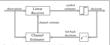
Figure 1 shows a simple DFE scheme. The main blocks are an adaptive channel estimation algorithm and a linear filter. The latter takes a channel estimate and the observa-tions at the receiver front-end to produce linear estimates of the transmitted symbols. These estimates are either real or complex numbers, depending on the modulation format. A threshold detector is used to convert them into hard symbol decisions, i.e., discrete estimates chosen from the symbol alphabet based on a minimum distance rule. We assume that the detector operates symbol-wise in order to keep the computational effort limited. The decisions at the output of the detector are fed back to the channel estimation block, so that they can be used to improve the subsequent channel estimates. Usually, the detected symbols are also employed to cancel inter-symbol interference (see, e.g., [8] and Section 3 in this article), but this is omitted in the figure for simplicity. We

observations Linear Receiver

symbol

estimates decisions

channel estimate

Channel Estimator

fed-back decisions

z− 1

Fig. 1Schematic representation of a DFE receiver. The figure illustrates the working a simple DFE receiver. The blockz−1 represents a delay of one symbol period

remark that the receiver is nonlinear, due to the threshold-ing operation, yet its computational complexity is similar to that of a linear receiver combined with an adaptive channel estimation algorithm [9], ([7] Chapter 16).

Any linear filter is amenable to be used in a DFE struc-ture. However, the use of the minimum mean square error (MMSE) filter has become widespread because it offers an attractive trade-off between noise amplification and inter-ference cancelation [10]. Many joint data detection and channel estimation algorithms (see, e.g., [11–14]) rely on the linear MMSE filter to carry out the equalization of an unknown MIMO channel. In every case, and to the best of our knowledge, the point estimatesof the chan-nel impulse response (CIR) provided by the corresponding estimator are used by the MMSE filter as if they were the trueCIR. However, the estimates are actually statistics of the true channel and, as such, have a mean and a covari-ance matrix, the latter measuring the uncertainty we have about their accuracy. When the Kalman filter (KF) [15, 16] is used to estimate the channel, both statistics, the mean and the covariance matrix of the channel become avail-able, but even then the usual approach (e.g., in [11, 17]) consists in taking the mean of the estimate as if it were the true channel and ignore the information provided by the covariance matrix. In this paper, we argue that significant performance gains can be expected by taking advantage of the second-order statistics (SOS) of the channel, with a low impact on the computational complexity of the receiver. To be specific, we show that reductions of several dBs in the signal-to-noise ratio (SNR) needed to attain a prescribed symbol error rate (SER) can be achieved using the proposed scheme. The main contributions of this work are the design and implementation of the new linear MMSE equalizer that exploits the second-order statistics of the channel, as well as extensive computer simulations showing the gains that can be expected from the proposed method as compared to the conventional one.

The remaining of this paper is organized as follows. In Section 2, the discrete-time baseband equivalent signal model of a MIMO transmission system with frequency-and time-selective channel is described. The stfrequency-andard

linear MMSE equalizer is briefly reviewed in Section 3. Our extension thereof using the channel SOS is intro-duced in Section 4. Section 5 outlines the DFE schemes resulting from the investigated equalizers. In Section 6, we show and discuss the results of extensive computer sim-ulations to compare the performance of the conventional DFE MMSE receiver (that ignores the channel SOS) and the proposed DFE SOS-MMSE scheme. Finally, Section 7 is devoted to the conclusions.

1.1 Summary of notation

Given a time-indexed sequence of (column) vectors,

xa,xa+1,· · ·,xb, we denote byxa_b the column vector con-structed by stacking, in order, all the vectors betweenxa andxb(including both), i.e.,

xa b =

x_a x_a+1 · · · x_b

.

An identity matrix of orderkis denoted byIk, whereas

0N,Mis anN×Mall-zeros matrix. IfN =M, we simply write0N. For a vectorx, x(i)represents itsith element, and given a matrixA,a(i)refers toith column.

2 Signal model

2.1 Time- and frequency-selective MIMO channel

We consider a MIMO communication system with Nt

transmitting antennas and Nr receiving antennas sepa-rated by a time- and frequency-selective (MIMO) channel. The discrete-time baseband-equivalent model describing the transmission can be written as (see, e.g., [18])

yt= m−1

i=0

Ht(i)st−i+gt, (1)

whereytis aNr×1 vector containing the observations col-lected at timet,mis the number of taps (usually referred to as the order) of the frequency-selective MIMO channel,

Ht(i)is the (time-varying)Nr×Ntchannel matrix associ-ated with theith tap,stis a vector of sizeNt×1 comprising the symbols transmitted at timet, andgtis anNr×1 vector of independent additive white Gaussian noise (AWGN) components with zero mean and varianceσ_g2.

Grouping the matrices associated with the different taps of the channel,Ht(i),i =0,. . .,m−1, in a singleoverall channel matrix,

Ht=[Ht(m−1) Ht(m−2) · · · Ht(0)] , (2)

of sizeNr ×Ntm, allows Eq. (1) to be written in a more compact form as

yt=Htst−m+1

t +gt, (3)

wherest−m+1

t is aNtm×1 vector that stacks all the symbol

vectors involved in thetth observation,

st−m+1

t =

s_t−m+1 s_t−m+2 · · · s_t

While non-standard, the notation in (4) shows explicitly that vectorst−m+1

t is constructed by stacking simpler

vec-tors in order and indicates the time indexes of the first (t−m+1 in this case) and last (there) elements to be stacked. These features should ease the understanding of some formulas in the sequel.

The evolution of the channel is modeled by means of an autoregressive (AR) process driven by white Gaussian noise1[11]. For the sake of generality, we consider an AR process of orderR, whose analytical description is given by

Ht= tically distributed (i.i.d.) Gaussian random variables (r.v.) with zero mean and varianceσ_v2.

Equations (3) and (5) can be seen, respectively, as the observation and state equations of a random dynamic system in state-space form. Since both equations are lin-ear and the corresponding noise processes are Gaussian, the Kalman filter (KF) can be applied to exactly compute the posterior probability distribution of the time-varying MIMO channel when the symbols are available.

In order to do so while using the standard KF equations, we first need to gather the whole state of the system (here, the channel at the last Rtime instants) in a single vec-tor and rewrite the state and observation equations in terms of it. MatrixHt can be represented as a vector in a straightforward manner by, e.g., stacking all its columns one upon another. In particular, if we letht(j)denote the jth column of matrixHt, then theNrNtm×1 vector

contains the same coefficients as matrix Ht. Using this vectorial notation and taking into account that, according to Eq. (5), the channel at a certain time instant depends on the channel at theRprevious time instants, the state of the system at timetcan be represented by the vector

ht−R+1

The state equation of the system can then be written in terms of thisaugmentedchannel vector as

ht−R+1

t =Qhtt−−R1 +vt, (8) wherevtis aNrNtmR×1 vector with i.i.d. Gaussian r.v.’s of zero mean and varianceσ_v2in the lastNrNtmpositions and zeros in the rest, and the state transition matrix,Q, is defined as

The observation (Eq. (3)) can also be easily rewritten in terms of the augmented channel vector,ht−R+1

t , as

We use the dynamic system in state-space form speci-fied by Eqs. (10) and (8) (which is equivalent to that given by Eqs. (3) and (5)) to track the unknown time-varying MIMO channel by means of a KF.

2.2 Stacked model

When a channel is time dispersive, a reliable detection of the transmitted symbols usually requires smoothing. It entails taking into account the observationsyt:t+d(the

parameter d ≥ 1 being the smoothing lag) in order to

detect the vectorstcontaining the symbols transmitted at timet. In such case, it is useful to consider an equation that relates a tall vector of stacked observations with the transmitted symbols, namely, which, at timet, have already been detected. It is conve-nient to identify their contribution to the stacked obser-vations vector,yt

t+d. Let us decompose the overall channel

where the submatricesH‡_t,d andHt,d encompass, respec-tively, the first Nt(m− 1) and last Nt(d + 1) columns ofHt,d. Then, the vector of stacked observations can be rewritten as

yt t+d =

H‡_t,d Ht,d

st−m+1

t−1

st t+d

+gt

t+d

=H‡_t,dst−m+1

t−1 +Ht,ds

t t+d+g

t t+d,

(15)

where the termH‡_t,dst−m+1

t−1 contains the contribution of the symbols transmitted up to timet−1, and can be treated as causal inter-symbol interference.

2.3 Kalman filtering

The KF [15] provides the optimal solution to the problem of estimating the state of a dynamic system in state-space form when its state and observation equations are linear and their corresponding noises are Gaussian.

In the problem at hand, the state of the system at time t is given by the augmented channel vector, ht−R+1

t , and

Eqs. (8) and (10) can be seen as, respectively, the state and observation equations of a dynamic system in state-space form. Since the above constraints of linearity and Gaussianity are met, the KF can be used to compute the probability density function of the state conditional on the available observations, p(ht−R+1

t |y0,· · ·,yt).

How-ever, the observation equation involves knowing, at time t, matrix St, which includes all the symbols transmitted between time instantst−m+1 andt. In practice, only

estimates of the symbols transmitted up to time t − 1

are available at time t, and hence we aim at the (pre-dictive) distribution of the state conditional on all the past observations and previously detected symbols, i.e., p(ht−R+1

t |y0,· · ·,yt−1,s˜0,· · ·,s˜t−1) with ˜st denoting the

vector containing the hard estimates of the symbols inst. Every expectation in the remaining of the paper is also (implicitly) conditional on the same information, and we denote it asEt−1[·]. For example, the posterior mean of the CIR at timet+k(k≥ 0) conditional ony0,· · ·,yt−1 ands˜0,· · ·,s˜t−1is written asEt−1[ht+k] and the poste-rior cross-covariance betweenht+kandht+k,k,k≥0, is denotedEt−1[ht+khH_t+k].

Notice that here the KF only yields an approximate solution insofar as it depends on the goodness of the previously detected symbols fed to it.

3 Linear MMSE smoothing

In order to detect the symbols transmitted at timetover a frequency-selective channel, it is usually a good approach to first remove the contribution of the already detected symbols from the observations vector [8]. At the sight of

Eq. (15), we can obtain causal-interference-free observa-tions as

zt

t+d:=ytt+d−H

‡

t,dstt−−m1+1 (16)

=Ht,dst

t+d+gtt+d. (17)

Computingzt

t+dfromy t

t+dentails knowing vectorstt−−m1+1, which encompasses symbol vectors st−m+1,· · ·,st−1. These are unknown but previous estimates thereof are available at timetand can be used as a surrogate. Hence, in practice, the stacked symbols vectorst−m+1

t−1 in Eq. (16) is replaced with vector,˜st−m+1

t−1 that contains hard estimates of the same symbols. This is a common approximation for the design of DFEs, and it usually makes sense under the assumption that the receiver is operating with a suf-ficiently low symbol error probability. Throughout the paper, we rely on this approximation, which amounts to taking the previously detected symbols as if they were the truly transmitted symbols, i.e.,

˜

st−m+1

t−1 =stt−−m1+1. (18) Assuming the causal interference is properly canceled, the linear MMSE estimation of the symbols transmitted at timetconsidering the observations up to timet+dcan be easily derived from Eq. (17) (see, e.g., [19]). In partic-ular, let theNr(d+1)×Nt(d+1) matrixFt represent the response of a linear system. Then, estimates of the transmitted symbols are computed as2

ˆ

st t+d=F

H t zt

t+d, (19)

and, in order to minimize the mean square error of these estimates, the response matrix can be computed by solv-ing the optimization problem

Ft=arg min Ft Et−1

FH_t zt

t+d−s t t+d

2

. (20)

Since the ultimate aim is to estimatestbut we are using observations up to timet+d, we refer to the linear

sys-tem whose response is given byFt in (20) as an MMSE

smoother.

Equation (20) poses a quadratic optimization problem and it is straightforward to obtain the closed-form solu-tion (see, e.g., [2])

FH_t =Et−1

st

t+dz

H

t

t+d Et−1

zt

t+dz

H

t t+d

−1

. (21)

observations, so that these are given by Eq. (17), then the expectations on the right-hand side of Eq. (21) can be shown to be

s denotes the variance of the symbols and it has been taken into account that the noise at timetis white and independent of the channel process and the symbols

transmitted up to t − 1, and that the channel and the

symbols are a priori independent.

The expectation on the right-hand side of Eq. (23) is usually approximated, to the best of our knowledge, by dealing with the channel matrixHt,das if it were a known given (deterministic) parameter, and hence

Et−1

Substituting (24) into Eq. (23) yields

Et−1

and combining Eqs. (22) and (25) in Eq. (21) yields the final expression for the response of the conventional linear MMSE smoother,

So far, we have assumed the channel is a known (deter-ministic) parameter. However, this is not usually the case in practice, and the common approach to tackle this prob-lem consists in replacing, whenever necessary, the (true) channel matrix with its expectation. Notice that here this entails a twofold approximation. On one hand, even when

assuming that the symbols up to timet −1 have been

detected exactly, at best one can only obtainapproximate causal-interference-free observations as On the other hand, taking the true channel matrix in Eq. (26) to be equal to its expectation results in the following approximation for the linear MMSE filter

FH_t ≈σ_s2Et−1

At the sight of Eqs. (13) and (14), in order to obtain Et−1

on the right-hand side of

Eqs. (27) and (28), respectively, we need the expecta-tions of the matrices Ht,Ht+1,. . .,Ht+d. At time t, the expectation of the channel matrixHtis given by the pre-dictive distribution of the KF, which takes into account the observations and symbols vectors up to timet−1. How-ever, the expectations of the matricesHt+1,. . .,Ht+dhave to be computed as well. In order to do so, we simply use Eq. (5) (the state equation of the system) to expand the expected channel matrix at timet, i.e.,

Et−1

4 MMSE smoothing using the channel SOS

The proposed MMSE detector treats the channel as an unknown (multidimensional) random variable (as opposed to a deterministic known parameter), and takes advantage of its second-order statistics rather than just its expectation. Additionally, it avoids performingexplicit interference cancelation, since this cannot be performed exactly. In order to do so, it aims to detect the transmitted symbols by solving the optimization problem

Ft=arg min

which is exactly the same as that posed by Eq. (20) replac-ingzt

Through straightforward algebraic manipulation, one can show

because the expectations are conditional on the previously detected symbols and we are assuming these match the truly transmitted ones (see Eq. (18) and the surrounding discussion).

4.1 The observation autocorrelation matrix

From Eq. (33), computing Et−1

amounts to the calculation ofEt−1

Et−1

. Regarding the first

expecta-tion, if we letht,d(j)denote thejth column of matrixHt,d andst

t+d(j)denote thejth element within vectors t t+d, then

the expectationEt−1

where the third equality follows because the symbols from timet onwards are a priori independent of the channel at timetand subsequent time instants, while the fourth equality holds because of the (also a priori) independence between different symbols, (assumed known), we have

Et−1

where, once again, we have used that the expectation is conditional on all the previously detected symbols and

hence, assuming these were exactly detected, vectorst−m+1

t−1 is known.

4.2 Channel cross-correlation matrices

Equations (34) and (36) involve computing the cross-correlation between different columns of matrices Ht,d andH‡_t,d, respectively. These are submatrices ofHt,d(see Eq. (14)), and hence their columns are ultimately columns from Ht,d. In particular, if we let ht,d(j) denote the jth

and every required cross-correlation is ultimately between columns ofHt,d. The structure of a column from the latter can be inferred from Eq. (13). Specifically, thejth column ofHt,dis given by

We compute the cross-correlation between any pair of columns in Ht,d, by way of their means and cross-the expectation of cross-the entire matrix, Ht,d, which can be obtained in a straightforward manner as explained at the end of Section 3. As for the cross-covariance_h

where_h˘ script are the same, this yields the (self-)covariance matrix h˘t+k(i),h˘t+k(i)=h˘t+k(i).

Recall from Eq. (40) thath˘t+k(i)fork = 0,· · ·,d, and i = 1,· · ·,Nr(d + 1), is either an all-zeros (column) vector or a column from matrixHt+k. Thus, when com-puting the cross-covariance between vectorsh˘t+k(i)and

˘

the cross-covariance between columnsnandqof matrix

Ht+k and can be obtained from the KF. Indeed, we can make the KF evolve from timetup to timet+kwhen no new information is available by takingkpredictive steps. This yields predictive statistics forht+k (a vectorial rep-resentation of Ht+k), and from its covariance matrix it is straightforward to obtain the cross-covariance matrix, ht+k(n),ht+k(q) between any pair of columnsht+k(n)and Appendix 7 for details) that, fork<l,

ht+k(n),ht+l(q)=

R

r=1

arht+k(n),ht+l−r(q), (45)

which allows for the recursive computation of the cross-covariance between any given two (different) columns in matricesHt,Ht+1,. . .,Ht+d. Notice that whenk > l, we can still use the above formula since

ht+k(n),ht+l(q)=

Since a KF estimating the augmented channel vector defined in Eq. (7) yields, at time t, the cross-covariance matrices hk(i),hl(j) with k,l = t − R + 1,. . .,t and

i,j = 1,. . .,Ntm, Eq. (45) allows the recursive com-putation of all the cross-covariance matrices needed to obtain, according to Eq. (42), the cross-covariance

matrix_h

t,d(i),ht,d(j), for any pair of columns in Ht,d. To

summarize,

• Equations (45), (42), and (41) together yield the channel cross-correlation matrices observation autocorrelation matrixEt₋1

4.3 The SOS-MMSE smoother

Having computed the stacked observations autocorrela-tion matrix given by Eq. (33), it is straightforward to plug it into Eq. (31), along with right-hand side of (32), to obtain the final expression for the proposed MMSE smoother that exploits the channel SOS explicitly,

FH_t =σ_s2Et−1HH_t,d

Notice that, at the sight of the right-hand side of Eq. (47), the proposed MMSE detector takes advantage of the pre-viously detected symbols. Hence, causal-interference can-celation is still being performed, although in an implicit manner (as opposed to the explicit causal-interference cancelation carried out by the conventional MMSE detector).

In order to ease the implementation of the proposed scheme, Pseudocode 1 gives an overview of the

neces-sary steps to obtain the MMSE smoother at timetwhen

the order of the AR process used to model the channel

dynamics is R = 1. The extension to higher order AR

processes is straightforward (the procedure is essentially the same), though some care is needed to build up the involved cross-covariance matrices in an adequate order.

Pseudocode 1Proposed SOS-MMSE smoother at timetwhenR=1 1: fork=1,· · ·,ddo

2: use KF equations over the dynamic system described by (10) and (8) withSt=0Nr×Ntmandyt=0Nr×1to get the predictive

mean,Hˆt+k := Et−1Ht+k, and covariance matrix,hˆt+k, ofHt+kgiven observations,y0,· · ·,yt−1, and the previously

detected symbols,s˜0,· · ·,˜st−1.

3: useHˆt,Hˆt+1,· · ·,Hˆt+dto build an estimate,Hˆt,d, ofHt,dusing (13) //computation ofEt−1

Ht,dst t+ds

H

t t+d

HH_t,d

4: setS←0

5: fori=1,· · ·,Nt(d+1)do

6: from Eq. (37) obtain the index,i, of the column within matrixHt,dsuch thatht,d(i)=ht,d(i) 7: initialize the covariance matrix for thei-th column of matrixHt,d:hˆt,d(i),hˆt,d(i)←0Nr(d+1)

8: fork=0,· · ·,ddo

9: from Eq. (40) obtain the indexnsuch thath˘t+k(i)=ht+k(n) 10: forl=k+1,· · ·,ddo

11: from Eq. (40) obtain the indexqsuch thath˘t+l(i)=ht+l(q) 12: ifh˘t+k(i)orh˘t+l(i)is0Nr×1then

13: continue to the next iteration of loop starting in line 10 14: obtain_hˆ

t+k(n),hˆt+k(q), the cross-covariance matrix between columnsnandqofHˆt+k by selecting the appropriate

coefficients from_hˆ_t+k

15: compute, according to Eq. (46),hˆt+k(n),hˆt+l(q)=a

l−k

1 hˆt+k(n),hˆt+k(q)

16: set_h˘

t+k(i),h˘t+l(i)←hˆt+k(n),hˆt+l(q)

17: inserth˘t+k(i),h˘t+l(i)(and its transpose ifk=l) into the adequate position of matrixhˆt,d(i),hˆt,d(i)according to (42)

18: obtainEt−1

ht,d(i)

as thei-th column ofHˆt,d

19: from_hˆ

t,d(i),hˆt,d(i)andEt−1

ht,d(i)

computeEt−1

ht,d(i)h H t,d(i)

according to (41)

20: setS←S+Et−1

ht,d(i)h H t,d(i)

//computation ofEt−1

H‡_t,dst−m+1

t−1 s H

t−m+1

t−1

H‡H_t,d

21: setS‡←0

22: fori=1,· · ·,Nt(m−1)do 23: forj=1,· · ·,Nt(m−1)do

24: initialize the cross-covariance matrix between thei-th andj-th columns of matrixHt,d:hˆt,d(i),hˆt,d(j)←0Nr(d+1)

25: fork=0,· · ·,ddo

26: from Eq. (40) obtain the indexnsuch thath˘t+k(i)=ht+k(n) 27: forl=0,· · ·,ddo

28: from Eq. (40) obtain the indexqsuch thath˘t+l(j)=ht+l(q) 29: ifh˘t+k(i)orh˘t+l(j)is0Nr×1then

30: continue to the next iteration of loop starting in line 27 31: ifk≤lthen

32: obtain_hˆ

t+k(n),hˆt+k(q), the cross-covariance matrix between columnsnandqofHˆt+kby selecting the appropriate

coefficients from_hˆ

t+k

33: else

34: obtain_hˆ

t+k(n),hˆt+k(q)as the transpose ofhˆt+l(q),hˆt+l(n), the cross-covariance matrix between columnsqandnof

ˆ

Ht+lby selecting the appropriate coefficients fromhˆt+l

35: compute, according to Eq. (46),_hˆ

t+k(n),hˆt+l(q)=a

|l−k|

1 hˆt+k(n),hˆt+k(q)

36: set_h˘

t+k(i),h˘t+l(j)←hˆt+k(n),hˆt+l(q)

37: insert_h˘

t+k(i),h˘t+l(j)into the adequate position of matrixhˆt,d(i),hˆt,d(j)

38: obtainEt−1

ht,d(i)

andEt−1

ht,d(j)

as, respectively, thei-th andj-th columns ofHˆt,d

39: from_hˆ

t,d(i),hˆt,d(j),Et−1

ht,d(i)

andEt−1

ht,d(j)

computeEt−1

ht,d(i)h H t,d(j)

according to (41)

40: setS‡←S‡+st−m+1

t−1 (i)stt−−1m+1(j) ∗_E

t−1

ht,d(i)h H t,d(j)

41: return FH

t =σs2Hˆt,d

σ2

sS+S‡+σg2INr(d+1)

ultimately the complexity of runningmKFs, each one esti-mating a state vector of lengthNrNtm(see lines 1–2 of Pseudocode 1). Therefore, the computational complexi-ties of the SOS-MMSE smoother and the conventional MMSE smoother of Section 3 are of the same order.

5 DFE schemes

The two MMSE smoothers described in Sections 3 and 4 can be readily used in a DFE scheme that relies on a Kalman filter for the channel tracking. In particular, we aim at comparing the performance of

• a conventional MMSE DFE that neglects the SOS generated by the KF, termed “MMSE + KF” in the sequel, and

• the proposed SOS-based MMSE DFE, termed “SOS-MMSE + KF”.

Figure 2 illustrates schematically the fundamental dif-ferences between the MMSE + KF- and SOS-MMSE + KF-based receivers. The KF yields the mean and the

interference

cancellation

channel mean

KF

MMSE

channel covariance matrix

z

·

·

channel mean

KF

SOS-MMSE

channel covariance matrix

z

·

·

(b)

(a)

Fig. 2Data exchange between the KF and theaMMSE + KF andb SOS-MMSE+KF receivers. The figure stresses the fundamental difference between the conventional MMSE and the one proposed. Notice how the channel matrix covariance given by the KF is fed to the smoother in thelowerfigure, whereas it is discarded in theupperone

covariance matrix of the channel impulse response, and both receivers make use of the former (along with the observations) to obtain estimates of the symbols transmit-ted. However, the proposed SOS-MMSE filter also takes advantage of the covariance matrix whereas the conven-tional MMSE neglects the information contained within this statistic. Also notice that the proposed receiver does not perform explicit interference cancelation (since this cannot be carried out exactly), as opposed to the conven-tional MMSE.

6 Simulation results

In order to assess the performance of the proposed algo-rithm, we have carried out computer simulations

con-sidering a system with Nt = 4 transmitting antennas

and Nr = 7 receiving antennas. The modulation

for-mat is BPSK and transmission is carried out in frames

of K = 300 symbol vectors (i.e., 1200 binary symbols

overall), including a training sequence of length T =

30 comprising symbols known to the receiver. This last parameter has been selected empirically, after observing that an increase thereof does not yield any noticeably per-formance improvement while decreasing it has indeed a negative impact. The training sequence is used at the beginning of each data frame to obtain a rough estimate of the channel impulse response. However, extending the method to use pilot symbols instead of, or in addition to, a training preamble is straightforward.

A flat power profile is assumed for the channel, and every coefficient is initially (and independently) drawn from a Gaussian distribution with zero mean and unit variance. As for the channel model, an AR process of order 1 has been considered, i.e.,R = 1. The coefficient of the AR process isa1=1−10−5, and we evaluate the perfor-mance of the MMSE + KF and SOS-MMSE + KF receivers in terms of the symbol error rate (SER) considering two different values for the variance of the channel noise,σ_v2, each one studied in a section of its own4. Furthermore, dif-ferent values for the channel order are explored in every case.

In all the simulations, each data frame is generated inde-pendently of all others (including the transmitted data, the MIMO channel realization and the noise terms), and the lag for the MMSE smoothers is set tod=m−1. The latter condition guarantees that every symbol is detected using all the related observations, and values of the smoothing lag abovem−1 do not seem to yield a noticeable per-formance gain. The results are averaged over 60, 000 data frames.

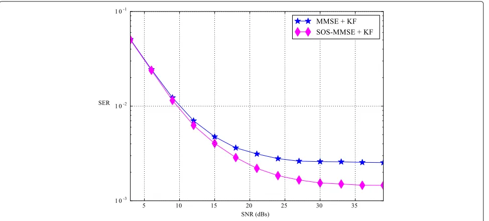
6.1 Slow fading channel (σ_v2=5×10−3)

Fig. 3SER for several values of the SNR (dB) with_σ2

v =0.005 andm=1

Figure 3 compares the SER achieved by the algorithms MMSE + KF and SOS-MMSE + KF for different values

of the SNR when the channel is flat (m = 1). In order

to reach a SER of 10−2, the method using the proposed MMSE DFE requires roughly 0.4 dBs less SNR than the method using the conventional MMSE DFE. This gap largely widens as the SNR increases: for a SER of 5×10−3, the curve for the MMSE + KF is more than 1 dB away from that of the SOS-MMSE + KF. Notice that both methods exhibit an error floor, but the one associated with the DFE scheme introduced in this paper is lower.

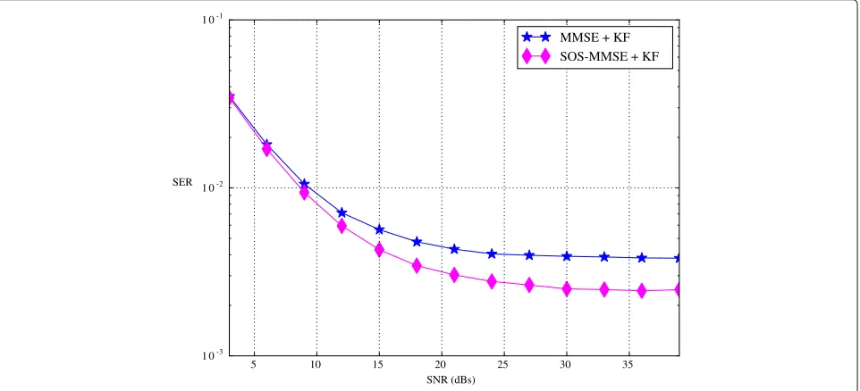
When the channel is flat, only the presentstate of the channel is needed (along with the observations) in order to detect the symbols transmitted. On the other hand, when the channel is dispersive, i.e., m > 1, not only does the number of channel coefficients to be estimated increase, but predictions offuturechannel states are also necessary in order to perform both causal-interference cancelation and smoothing. Overall, this results in less reliable channel estimates being employed, and hence accounting for their uncertainty becomes important. This is illustrated in Fig. 4 that shows the performance of the

5 10 15 20 25 30 35

SNR (dBs) 1 0-3

1 0-2 1 0-1

SER

MMSE + KF SOS-MMSE + KF

Fig. 4SER for several values of the SNR (dB) withσ2

5 10 15 20 25 30 35 SNR (dBs)

1 0-4 1 0-3

1 0-2 1 0-1

1 00

SER

MMSE + KF SOS-MMSE + KF

Fig. 5SER for several values of the SNR (dB) withσ2

v =0.005 andm=5

algorithms whenm = 3. When comparing these results

to those obtained form = 1, the SER achieved by the

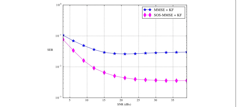
MMSE + KF degrades over the whole range of SNRs on account of this algorithm neglecting the channel SOS. On the other hand, the SOS-MMSE + KF is able to success-fully cope with the uncertainty in the channel estimates and even sees a performance boost due to the increase in diversity given by a higher channel order. As a conse-quence, the proposed receiver now exhibits a more clear advantage over the conventional one. Indeed, in order to attain a SER of 10−2, the latter requires around 2.4 dBs more SNR than the former. Figure 5 shows that when

the channel order ism = 5, the gap between the curves of the SOS-MMSE + KF and MMSE + KF algorithms widens even more. Moreover, the performance of the SOS-based MMSE DFE improves slightly whereas that of the conventional MMSE DFE further deteriorates.

6.2 Fast fading channel (σ_v2=0.01)

Increasing the variance of the channel noise has a twofold effect. On one side, since the channel now changes more rapidly and hence it is harder to track, the performance of any receiver is expected to worsen. On the other side, the channel evolving faster means that predictions about

5 10 15 20 25 30 35

SNR (dBs) 1 0-3

1 0-2 1 0-1

SER

MMSE + KF SOS-MMSE + KF

Fig. 6SER for several values of the SNR (dB) withσ2

5 10 15 20 25 30 35 SNR (dBs)

1 0-3 1 0-2 1 0-1

SER

MMSE + KF SOS-MMSE + KF

Fig. 7SER for several values of the SNR (dB) withσ2

v =0.01 andm=3

its future state are less reliable, and hence accounting for their uncertainty is even more important (which should benefit the SOS-based MMSE DFE). From a mathemat-ical point of view, if the predicted channel estimates are not accurate, then the elements in the covariance matrices that enter Eq. (41) are non-negligible and so is their con-tribution to the computation of the proposed MMSE DFE in Eq. (47).

Figure 6 shows the performance of the algorithms in a

flat channel (m = 1). The SER of both DFEs degrades

in the medium-high SNR region, as compared to the pre-vious scenario, but this penalty is larger in the case of

the MMSE + KF. Thus, the proposed MMSE DFE now exhibits a more pronounced advantage over the conven-tional MMSE (about 0.65 dBs for a SER of 10−2and more than 3 dBs for a SNR of 5×10−3).

Increasing the channel order in a fast fading channel has a negligible effect on the performance of the

SOS-MMSE + KF5 but seriously harms that of the MMSE +

KF. In Fig. 7, it can be seen that, when the channel

order is m = 3, a SER of 10−2 requires ≈ 8.3 dBs

less SNR in the former than in the latter (recall that in the previous scenario this gap was approximately 2.4 dBs).

5 10 15 20 25 30 35

SNR (dBs) 1 0-3

1 0-2 1 0-1 1 00

SER

MMSE + KF SOS-MMSE + KF

Fig. 8SER for several values of the SNR (dB) withσ2

Results for the case in whichm=5 are shown in Fig. 8. Again, the advantage of the proposed method over the conventional one is much more clear as the channel order increases.

7 Conclusions

In this work, we have introduced an enhanced version of the conventional MMSE equalizer for time-selective MIMO channels that takes advantage of the posterior second-order statistics of the channel provided by the KF. Computer simulations show that the proposed SOS-MMSE DFE yields significant performance gains (in terms of SER) over the conventional MMSE in the medium-high SNR region. In medium-highly dispersive channels, the SNR required for the proposed SOS-MMSE receiver to achieve a certain SER can be several dBs lower than that required by the conventional MMSE. This is especially true for fast-varying channels, in which the uncertainty about the channel estimates becomes important. Indeed, a mea-sure of this uncertainty is given by the second-order statistics of the channel, which are dismissed by the con-ventional MMSE, but handled by the one introduced in this paper.

It is important to point out that the application of the SOS-aided MMSE filter introduced in this work is not restricted to DFE receivers. On the contrary, the key idea is very general and can be integrated into any MMSE-based scheme as long as SOS of an unknown random variable that is relevant for the filter (here, the channel) are available.

One last remark is that the computational complexity of the proposed SOS-MMSE DFE is of the same order as that of the conventional scheme that neglects the channel SOS.

Endnotes

1_{For all practical purposes, any model that is linear and}

affected by Gaussian noise is amenable to be used here. 2_{Notice that (for the sake of mathematical convenience)}

estimates of the symbol vectors st+1,st+2,· · ·,st+d are obtained at timet(using observations up to timet+d) since they are also included in st

t+d. However, they are

dismissed at that time and the actual estimates of the symbols in st+i are computed at time t + i using the observations up to timet+i+d.

3_{This is a reasonable hypothesis since the smoothing lag}

should be selected to account for, at least, the observa-tions containing all the energy of the symbols transmitted at timet. This obviously depends on the length of the CIR, m, and it is common to set the smoothing lag tod=m−1. This is also the case in the experiments whose results are presented in Section 6.

4_{Notice that the higher the variance of the channel}

noise, the more rapidly the channel coefficients fluctu-ate. A faster varying channel can also be obtained by decreasing the coefficient of the AR process,a1, which determines the correlation between a channel coefficient and itself at a different time instant.

5_{Here, the increase in diversity due to a higher channel}

order is not enough to compensate for the rapid variation of the channel coefficients.

Appendix

Computation of the cross-covarianceht+k(n),ht+l(q) withk<l

Theqth column in matrixHt+l,ht+l(q), can be expressed, according to Eq. (5), as

ht+l(q)= ables (r.v.) with zero mean and varianceσ_v2. Its expectation is then given by

Et−1

Notice that this last equation is just Eq. (29) restated column-wise.

Substituting Eqs. (48) and (49) into (43), we obtain

ht+k(n),ht+l(q)=Et−1

Since we are assuming k < l, it is clear from

since Et₋1

ht+k(n)

is a constant. Therefore, Eq. (50) becomes

(and through straightforward algebraic manipulation)

=

Since all the terms in the second summation of (51) are zero, only the first summation is left and the equation can be rewritten as

where Eq. (44) has been used in the last step of the derivation.

Abbreviations

AWGN: Additive white Gaussian noise; AR: Autoregressive; BPSK: Binary phase-shift keying; CIR: Channel impulse response; DFE: Decision feedback equalizer; i.i.d.: Independent and identically distributed; KF: Kalman filter; MIMO: Multiple input multiple output; MMSE: Minimum mean square error; r.v.: Random variable; SOS: Second-order statistics; SER: Symbol error rate

Acknowledgements

This work was supported byMinisterio de Economía y Competitividadof Spain (project COMPREHENSION TEC2012-38883-C02-01),Comunidad de Madrid (project CASI-CAM-CM S2013/ICE-2845), and the Office of Naval Research Global (award no. N62909- 15-1-2011).

Competing interests

The authors declare that they have no competing interests.

Author details

1_{Departamento de Teoría de la Señal y Comunicaciones, Universidad Carlos III} de Madrid, Avenida de la Universidad 30, Leganés, Spain.2_{School of} Mathematical Sciences, Queen Mary University of London, Mile End Road, E1 4NS, London, UK.3_{Gregorio Marañón Health Research Institute, Calle del Dr.} Esquerdo, 46, 28007 Madrid, Spain.

Received: 26 April 2016 Accepted: 8 November 2016

References

1. E Telatar, Capacity of multi-antenna Gaussian channels. Eur. Trans. Telecommun.10, 585–595 (1999)

2. S Verdú,Multiuser Detection. (Cambdridge University Press, Cambridge, 1998)

3. TS Rappaport,Wireless Communications: Principles and Practice, (2nd Edition). (Prentice-Hall, Upper Saddle River, 2001)

4. C Tidestav, A Ahlen, M Sternad, Realizable MIMO decision feedback equalizers: structure and design. IEEE Trans. Signal Process.49(1), 121–133 (2001)

5. CA Belfiore, JH Park Jr., Decision feedback equalization. Proc. IEEE.67(8), 1143–1156 (1979)

6. AH Sayed,Adaptive Filters. (Wiley-IEEE Press, Hoboken, 2008) 7. AF Molisch,Wireless Communications, vol. 15. (John Wiley & Sons, West

Sussex, 2010)

8. JG Andrews, Interference cancellation for cellular systems: a contemporary overview. Wireless Commun. IEEE.12(2), 19–29 (2005) 9. AM Chan, GW Wornell, A new class of efficient block-iterative interference

cancellation techniques for digital communication receivers. J. VLSI Signal Process. Syst. Signal Image Video Technol.30(1-3), 197–215 (2002) 10. E Biglieri, AR Calderbank, AG Constantinides, A Goldsmith, A Paulraj,

MIMO Wireless Communications. (Cambridge University Press, Cambridge, 2010), p. 1323

11. C Komnikakis, C Fragouli, AH Sayed, RD Wesel, Multi-input multi-output fading channel tracking and equalization using Kalman estimation. IEEE Trans. Signal Process.50(5), 1065–1076 (2002)

12. J Choi, Equalization and semi-blind channel estimation for space-time block coded signals over a frequency-selective fading channel. IEEE Trans. Signal Process.52(3), 774–785 (2004)

13. MA Vázquez, MF Bugallo, J Míguez, Sequential Monte Carlo methods for complexity-constrained MAP equalization of dispersive MIMO channels. Signal Process.88, 1017–1034 (2008)

14. G Yanfei, H Zishu, inCommunications, Circuits and Systems, 2005. Proceedings. 2005 International Conference On. MIMO channel tracking based on Kalman filter and MMSE-DFE, vol. 1 (IEEE, 2005), pp. 223–226 15. RE Kalman, A new approach to linear filtering and prediction problems.

J. Basic Eng.82, 35–45 (1960)

16. BDO Anderson, JB Moore,Optimal filtering. (Englewood Cliffs, New Jersey, 1979)

17. N Al-Dhahir, AH Sayed, The finite-length multi-input multi-output MMSE-DFE. Signal Process. IEEE Trans.48(10), 2921–2936 (2000) 18. D Guo, X Wang, Blind detection in MIMO systems via sequential Monte

Carlo. IEEE J. Selected Areas Commun.21(3), 464–473 (2003)

19. J Míguez, L Castedo, Space-time channel estimation and soft detection in time-varying multiaccess channels. Signal Process.83(2), 389–411 (2003)

Submit your manuscript to a

journal and benefi t from:

7Convenient online submission 7Rigorous peer review

7Immediate publication on acceptance 7Open access: articles freely available online 7High visibility within the fi eld

7Retaining the copyright to your article