R E S E A R C H
Open Access
A high-order numerical scheme using
orthogonal spline collocation for solving the
two-dimensional fractional
reaction–subdiffusion equation
Xiaoyong Xu
1,2and Da Xu
1**Correspondence: [email protected] 1College of Mathematics and
Statistics, Hunan Normal University, Changsha, P.R. China
Full list of author information is available at the end of the article
Abstract
In this paper, a high-order numerical scheme is proposed for solving the
two-dimensional fractional reaction–subdiffusion equation. The method is based on adopting a third-order weighted and shifted Grünwald difference (WSGD) operator to approximate the time Caputo fractional derivative and applying the orthogonal spline collocation (OSC) method to approximate the spatial derivative. Stability and convergence analysis of the proposed method are rigorously proved. Several numerical examples in one variable and in two space variables are presented to validate our theoretical analysis.
MSC: 35R11
Keywords: Two-dimensional reaction–subdiffusion equation; Orthogonal spline collocation; WSGD operator; Caputo derivative; Stability; Convergence
1 Introduction
Fractional equations can be used to describe some physical phenomenon more accurately than the classical integer-order differential equation, one of which fractional reaction– diffusion equations have been researched in recent years in many areas of science and en-gineering. A fractional reaction–subdiffusion equation can be derived from a continuous time random walk model when the transport is dispersive [1] or a continuous time random walk model with temporal memory and sources [2]. The analytical solutions of such equa-tions are usually difficult to obtain, so seeking numerical soluequa-tions becomes more impor-tant and emergent. These numerical methods mainly covers compact difference methods [3–5], finite element methods [6,7], spectral methods [8,9], meshless methods [10,11], the homotopy analysis method [12], the Legendre operational matrix method [13], and spline collocation methods [14–16].
Although there are many studies on numerical methods for one-dimensional frac-tional partial differential equations, there are few studies on numerical methods for two-dimensional time fractional differential equations, when compared with one-two-dimensional problems. Huang [17] proposed a numerical algorithm for a two-dimensional fractional reaction subdiffusion equation withτ1+γorder in time and second order in space. Yu [18]
considered a numerical method for the two-dimensional non-linear fractional reaction– subdiffusion equation, which is of second-order temporal accuracy and fourth-order spatial accuracy. In [19], Yang developed novel numerical techniques for the solution of the two-dimensional fractional sub-diffusion equation, which is based on the or-thogonal spline collocation method in space and a finite difference method (FDM) in time. Ömer et al. [20] established a wavelet method, based on Haar wavelets and a fi-nite difference scheme for the two-dimensional time fractional reaction–subdiffusion equation. Li [21] proposed a numerical treatment for two-dimensional fractional sub-diffusion equations using the parametric quintic spline. In [22], Dehghan used the dual reciprocity boundary elements method for the numerical solution of two-dimensional linear and nonlinear time-fractional modified anomalous subdiffusion equations and time-fractional convection-diffusion equation. Bhrawy and Zaky applied spectral tau and collocation methods for different kinds of fractional partial differential equations in the multi-dimensional case [23–27].
In this study, we consider the following two-dimensional time fractional reaction– subdiffusion equation:
C
0D
α
tu(x,y,t) =Kαu(x,y,t) –Cαu(x,y,t) +f(x,y,t), (x,y,t)∈Ω×(0,T] (1.1) subject to the initial condition
u(x,y, 0) =φ(x,y), (x,y)∈Ω, (1.2)
and the boundary condition
u(x,y,t) = 0, (x,y,t)∈∂Ω×(0,T], (1.3)
where is Laplace operator,Ω= [0, 1]×[0, 1] with boundary∂Ω, Kα > 0 is diffusion coefficient,Cα> 0 is the constant reaction rate, andC0Dαt denotes the Caputo derivative of
orderα(0 <α< 1), which reads as follows:
C
0D
α
tu(x,y,t) =
1 Γ(1 –α)
t
0
∂u(x,y,s) ∂s (t–s)
–α
ds,
in whichΓ(·) is the Gamma function.
the integer and fractional derivatives in time are discretized by second-order two-step backward difference method and second-order WSGD operator. In [33], Yang discussed a new numerical approximation for the two-dimensional distributed-order time fractional reaction–diffusion equation, which combines the idea of a WSGD operator with the sec-ond order in time direction and the orthogonal spline collocation method in the space direction.
The orthogonal spline collocation (OSC) method has developed into a robust and valu-able technique for solving many kinds of partial differential equations [34–38]. The pop-ularity of OSC is due to its simple concept, wide applicability and easy implementation. Comparing with the finite difference method [39] and the Galerkin finite method [40], the OSC method has the following advantages: the calculation of the coefficients in the equation determining the approximate solution is fast since there is no need to calculate the integrals; and it provides approximations to the solution and spatial derivatives. More-over, the OSC method always leads to the almost block diagonal linear system, which can be solved by the software packages efficiently [41]. Another feature of the OSC method lies in its super-convergence [42].
Inspired and motivated by the work mentioned above, the main purpose of this paper is to propose a high-order OSC approximation method combined with a third-order WSGD operator to solve a two-dimensional fractional reaction–subdiffusion equation, abbrevi-ated WSGD-OSC in forthcoming sections.
The rest of the paper is organized as follows. In Sect.2, we introduce some notations and preliminaries. In Sect.3, the fully discrete scheme combined with a WSGD operator with third order and an orthogonal spline collocation scheme is constructed. Stability and con-vergence analyses of the WSGD-OSC scheme are presented in Sect.4. Section5presents detailed description of the WSGD-OSC scheme. In Sect.6, numerical experiments are carried out to confirm the convergence analysis. Finally, the conclusion is drawn in Sect.7.
2 Preliminaries
In this section, we will introduce some notations and basic lemmas. For some positive integersNxandNy,πxandπyare two uniform partitions ofI= [0, 1] which are defined as
follows:
πx: 0 =x0<x1<· · ·<xNx= 1, πy: 0 =y0<y1<· · ·<yNy= 1,
andhxi =xi–xi–1,Iix= (xi–1,xi), 1≤i≤Nx, andhyj =yj–yj–1, Ijy= (yj–1,yj), 1≤j≤Ny,
h=max(max1≤i≤Nxh
x
i,max1≤j≤Nyh
y
j). Let Mr(πx) andMr(πy) be the space of piecewise
polynomials of degree at mostr≥3, defined by
Mr(πx) =
v∈C1[0, 1] :v|Iix∈Pr, 1≤i≤Nx,v(0) =v(1) = 0
,
Mr(πy) =
v∈C1[0, 1] :v|Iy
j ∈Pr, 1≤j≤Ny,v(0) =v(1) = 0
,
wherePrdenotes the set of polynomial of degree at mostr. It is easy to know that the
dimension of the spacesMx(πx) andMy(πy) are (r– 1)Nx:=Mxand (r– 1)Ny:=My,
re-spectively.
Letπ=πx⊗πybe a quasi-uniform partition ofΩ, andMr(π) =Mr(πx)⊗Mr(πy) with
quadrature rule on the intervalIwith corresponding weights{ωj}rj=1–1. Denote by
the sets of Gauss points inxandydirection, respectively, where
ξix,l=xi–1+hxiλl, ξjy,m=yj–1+hyjλm, 1≤l,m≤r– 1.
LetG={ξ = (ξx,ξy) :ξx∈Gx,ξy∈Gy}. For the functionsuandvdefined onG, the inner
productu,vand normvMr are, respectively, defined by
u,v=
Forma nonnegative integer, letHm(Ω) denote the usual Sobolev space with norm
vHm= venience. The following important lemmas are required in our forthcoming analysis. First, we introduce the differentiable (resp. twice differentiable) mapW: [0,T]→Mr(π) by
(u–W) = 0 onG×[0,T], (2.1)
whereuis the solution of Eqs. (1.1)–(1.3). Then we have the following estimates foru–W
and its time derivatives.
Lemma 2.1([34]) If∂lu/∂tl∈Hr+3–j,for all t∈[0,T],l= 0, 1, 2,j= 0, 1, 2,and W is defined by(2.1),then there exists a constant C such that
and there exists a positive constant C such that
Lemma 2.4([44]) The norms · Mrand · are equivalent on Mr(π).
Throughout the paper, we denoteC> 0 a constant which is independent of space–time mesh sizeshandτ. It is not necessarily the same on each occurrence. Besides, the following Young inequality will be used repeatedly:
de≤εd2+ 1 4εe
2, d,e∈R,ε> 0. (2.6)
3 Construction of the fully discrete orthogonal spline collocation scheme
For the analysis, we need to introduce the Riemann–Liouville fractional derivative and Liouville fractional derivative of orderα(0 <α< 1) for a functionu(t), which are defined by
RL
0 D
α
tu(t) =
1 Γ(1 –α)
d dt
t
0
u(τ)
(t–τ)αdτ (3.1)
and
–∞Dαtu(t) =
1 Γ(1 –α)
d dt
t
–∞
u(τ)
(t–τ)αdτ. (3.2)
Lemma 3.1([30]) If f ∈C(2+m)(R),then f ∈Lα+m(R),for anyα∈(0, 1),where the space is
defined asLα+m(R) ={f| ∞
–∞(1 +ω)
α+mˆf(ω)dω< +∞,f is the Fourier transform of fˆ }.
Lemma 3.2([45]) For any f∈L1(R)∩Lα+1(R),we define the shifted Grünwald difference
operator
A(τα,p)f(t) =
1 τα
∞
k=0
gk(α)ft– (k–p)τ, (3.3)
where p is a non-positive and gk(α)= (–1)kα
k
zk= Γ(k–α)
Γ(–α)Γ(k+1).Then
A(τα,p)f(t) =–∞Dαtf(t) +O(τ). (3.4)
Lemma 3.3([28]) Let f(t),–∞Dtα+3f(t)and its Fourier transformf belong to Lˆ 1(R).Define
the weighted and shifted Grünwald difference operator by
Dατf(t) =ρ1Aτ(α,p)f(t) +ρ2Aτ(α,q)f(t) +ρ3Aτ(α,r)f(t), (3.5)
where
ρ1=
12qr– (6q+ 6r+ 1)α+ 3α2
12(qr–pq–pr+p2) , ρ2=
12qr– (6q+ 6r+ 1)α+ 3α2 12(pr–pq–qr+q2) ,
ρ3=
12qq– (6p+ 6q+ 1)α+ 3α2 12(pq–pr–pqr+r2) ,
and p,q and r are all integers.Then we have
Dατf(t) =–∞Dαtf(t) +O
uniformly for t∈Rasτ→0.We consider the case p>q>r and choose(p,q,r) = (0, –1 – 2), to the relationship between the Caputo derivative and the Riemann–Liouville fractional derivative,we have
time OSC schemes for solving Eqs. (1.1)–(1.3). The continuous-time OSC scheme to the solutionuof (1.1) is a differentiable mapuh: (0,T]→Mr(π) such that
shifted Grünwald difference operator to approximateC
0Dαtu(x,y,t), without loss of
gener-ality we assumeu(x,y, 0) = 0, otherwise, we may consider a transformu(x,y, 0) =u(x,y, 0) – ϕ(x,y), thenC
0Dαtu(x,y,t) =0RLDαtu(x,y,t). According to Theorem 1 in [28], we can obtain
the following estimate of the truncation error.
Lemma 3.4 Suppose∀α> 0,andRL
For the sake of convenience, we use the symbolDα
(3.6), the full-discrete WSGD-OSC scheme for (1.1) consists in finding{un
h}Kn=0⊂Mr(π)
such that
Dατunh–Kαunh+Cαunh=fhn, n= 0, 1, . . . ,K. (3.10)
4 Stability and convergence analysis of the WSGD-OSC scheme
In this section, we will give the stability and convergence analysis for fully discrete WSGD-OSC scheme (3.10). To this end, we further need the following lemma.
Lemma 4.1([30]) Let{q(kα)}∞k=0de defined in(3.7).Ifα∈(0,α∗],then,for any positive
in-Theorem 4.1 The fully discrete WSGD-OSC scheme(3.10)is unconditionally stable for sufficiently smallτ> 0;we have
Cατ
Taking advantage of the Cauchy–Schwarz inequality to the right hand side (RHS) of (4.5),
using Lemma2.2and the Young inequality, the second term in the RHS of (4.12) can be
Applying the Young inequality and (4.11), the last term in (4.12) can be estimated as
Finally, in order to estimate the first term on the RHS of (4.12), we first define a new elliptic projectionW of the exact solutionubyW: [0,T]→Mr(π) by
0RLDαtu–W = 0 onG×[0,T], (4.15)
then, from Theorem 3.4 in [46], it follows that
RL
by introducingρdefined by
–ρ=RL0 Dα
tW–W, inΩ×[0,T],
ρ= 0, on∂Ω×[0,T].
According to the proof of Lemma 3.5 in [34], and a straightforward modification of the argument given in the proof of Theorem 2.1 of [47], we can obtain
RL
using the triangle inequality and combining (4.16) and (4.17), we can obtain
Substituting (4.13)–(4.14) and (4.19) in (4.12), then summing (4.12) fromn= 0 ton=
Therefore, using the triangle inequality and Lemmas2.1–2.2and2.4, (4.20) then yields
the desired result.
5 Description of the WSGD-OSC scheme
It can be seen from the fully discrete scheme (3.10) that we need to solve a partial differ-ential equation with two variables at each time level, that is,
τ–α
For implementing the numerical schemes, we usually first representun
hby the base
func-tions ofMr(π), then solve the coefficients of the representation formula. More concretely,
letting
i,j=1 are unknown coefficients to be determined. Setting
ˆ
u=uˆn1,1,uˆ1,2n , . . . ,uˆn1,My,uˆn2,1,uˆn2,2, . . . ,uˆnMx,MyT
where
We implement the WSGD-OSC scheme in the piecewise Hermite cubic spline space
M3(π).
It is very natural that we choose cubic Hermite polynomials for satisfying the zero boundary condition. In detail, we choose the basis of cubic Hermite polynomial, namely, for 1≤i≤N– 1, it follows that
ψi(1) = 0. Renumber the basis functions; let
{ψ0,φ1,ψ1,φ2, . . . ,φN–1,ψN–1,ψN}={Φ1,Φ2,Φ3, . . . ,Φ2N},
then
Mr(πx) =span{Φ1,Φ2,Φ3, . . . ,Φ2N}, Mr(πy) =span{Φ1,Φ2,Φ3, . . . ,Φ2N}.
we find the formula for the values of the basis function at the Gauss point and the second derivatives. They are defined as follows:
H1(uj) = (1 + 2uj)(1 –uj)2, H2(uj) =uj(1 –uj)2hk,
3)/6. With the above descriptions on the basis function, we give an example of the matrixBx andAx in the case ofNm= 5 andhk= 1/Nm. We
It is well known from the tensor product calculation results that the WSGD-OSC scheme requires the solution of an almost block diagonal linear system at each time step. This system can be solved efficiently using the software package COLROW [41].
6 Numerical experiments
In this section, several numerical examples are given to illustrate our theoretical analysis. In our implementations, we adopt the space of piecewise Hermite cubic with the standard value and scaled slope basis functions [48] on uniform partitions ofIin both thexand
ydirections withNx=Ny=N. The forcing termf(x,y,t) is approximated by the
piece-wise Hermite interpolant projection in the Gauss collocation point. In order to check the accuracy of the proposed method, we present theL∞andL2errors atT= 1 and the cor-responding rates of convergence defined by
Convergence rate≈ log(em/em+1)
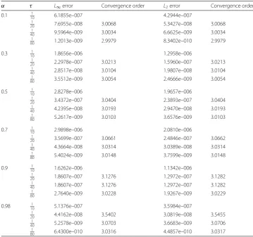
Table 1 TheL∞,L2errors and temporal convergence orders withh= 1/1000 for Example1
α τ L∞error Convergence order L2error Convergence order
0.1 101 6.1855e–007 4.2944e–007
1
20 7.6955e–008 3.0068 5.3427e–008 3.0068
1
40 9.5964e–009 3.0034 6.6625e–009 3.0034
1
80 1.2013e–009 2.9979 8.3402e–010 2.9979
0.3 1
10 1.8656e–006 1.2958e–006
1
20 2.2978e–007 3.0213 1.5960e–007 3.0213
1
40 2.8517e–008 3.0104 1.9807e–008 3.0104
1
80 3.5512e–009 3.0054 2.4666e–009 3.0054
0.5 101 2.8278e–006 1.9657e–006
1
20 3.4372e–007 3.0404 2.3893e–007 3.0404
1
40 4.2395e–008 3.0193 2.9470e–008 3.0193
1
80 5.2617e–009 3.0103 3.6576e–009 3.0103
0.7 101 2.9898e–006 2.0810e–006
1
20 3.5699e–007 3.0661 2.4846e–007 3.0662
1
40 4.3664e–008 3.0314 3.0389e–008 3.0314
1
80 5.4024e–009 3.0148 3.7599e–009 3.0148
0.9 1
10 1.6262e–006 1.1342e–006
1
20 1.8607e–007 3.1276 1.2972e–007 3.1282
1
40 1.8607e–007 3.1276 1.2972e–007 3.1282
1
80 2.7640e–009 3.0228 1.9267e–009 3.0229
0.98 101 5.1376e–007 3.5984e–007
1
20 4.4162e–008 3.5402 3.0819e–008 3.5455
1
40 5.2578e–009 3.0703 3.6683e–009 3.0706
1
80 6.4300e–010 3.0316 4.4857e–010 3.0317
whereh= 1/Nmis the time step size withN=Nm, andemis the norm of the corresponding
error.
Example1 As the first example, we consider the following one-dimensional fractional reaction–subdiffusion equation:
c
0D
α
tu(x,t) =
∂2u(x,t)
∂x2 –u(x,t) +f(x,t), 0 <x< 1, 0 <t≤1,
u(x, 0) = 0, 0≤x≤1, (6.1)
u(0,t) = 0,u(1,t) = 0, 0≤t≤1,
where f(x,t) = (ΓΓ(4–(4)α)t3–α+t3)x2(1 –x)2ex–t3ex(2 – 8x+x2+ 6x3+x4). The analytical solution of this equation isu(x,t) =t3x2(1 –x)2ex.
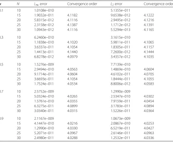
Table 2 TheL∞,L2errors and spatial convergence orders withτ= 1/1000 for Example1
α h L∞error Convergence order L2error Convergence order
0.1 101 3.4339e–006 2.5064e–006
1
20 2.1541e–007 3.9947 1.5705e–007 3.9963
1
40 1.3497e–008 3.9964 9.8209e–009 3.9992
1
80 8.4315e–010 4.0007 6.1352e–010 4.0007
0.3 1
10 3.1758e–006 2.3248e–006
1
20 1.9975e–007 3.9909 1.4568e–007 3.9962
1
40 1.2499e–008 3.9983 9.1095e–009 3.9993
1
80 7.7988e–010 4.0024 5.6827e–010 4.0027
0.5 101 2.8749e–006 2.1134e–006
1
20 1.8151e–007 3.9854 1.3245e–007 3.9960
1
40 1.1350e–008 3.9993 8.2822e–009 3.9993
1
80 7.0704e–010 4.0048 5.1598e–010 4.0046
0.7 101 2.5405e–006 1.8696e–006
1
20 1.6044e–007 3.9850 1.172e–007 3.9957
1
40 1.0032e–008 3.9994 7.3288e–009 3.9993
1
80 6.2455e–010 4.0056 4.5634e–010 4.0054
0.9 1
10 2.1719e–006 1.5897e–006
1
20 1.3618e–007 3.9954 9.9689e–008 3.9952
1
40 8.5366e–009 3.9957 6.2348e–009 3.9990
1
80 5.3234e–010 4.0032 3.8885e–010 4.0031
0.98 101 2.0086e–006 1.4663e–006
1
20 1.2597e–007 3.9950 9.1972e–008 3.9948
1
40 7.8801e–009 3.9987 5.7531e–009 3.9988
1
80 4.9259e–010 3.9998 3.5943e–010 4.0006
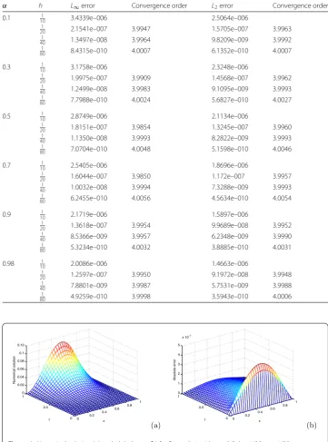
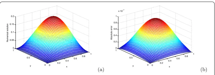
Figure 1Numerical solution (a) and global error (b) for Example1withα= 0.5,h= 1/32,τ= 1/32
τ = 1/1000 is fixed. The numerical solution and the global error forα= 0.5, h= 1/32,
τ = 1/32 are shown in Fig.1.
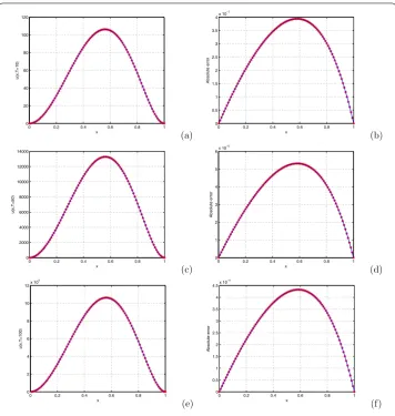
Figure 2The exact solution and numerical solution at different time (T= 10, 50, 100) withα= 0.5,h= 1/100,
τ= 1/100 and corresponding error for Example1. Dotted line: numerical solution, solid line: exact solution
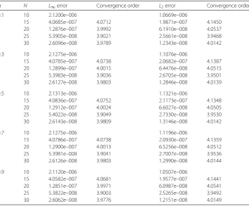
Example 2 Consider the following two-dimensional fractional reaction–subdiffusion equation:
c
0D
α
tu(x,y,t) –u(x,y,t) +u(x,y,t) =f(x,y,t),
u(x,y, 0) = 0, (x,y)∈Ω, (6.2)
u(x,y,t) = 0, (x,y,t)∈∂Ω×(0,T],
whereΩ= [0, 1]×[0, 1],T= 1,f(x,y,t) = [ΓΓ(4–(4)α)t–α(1 –x)(1 –y) – (3x+ 3y+xy– 7)]t3xyex+y.
The exact solution of the equation isu(x,y,t) =t3xy(1 –x)(1 –y)ex+y.
Table 3 TheL∞,L2errors and temporal convergence orders for Example2
α N L∞error Convergence order L2error Convergence order
0.1 10 2.1115e–006 1.2466e–006
15 4.3256e–007 3.9102 2.7478e–007 3.7296
20 1.5178e–007 3.6404 9.6187e–008 3.6487
25 6.9421e–008 3.5056 4.3264e–008 3.5805
30 3.7137e–008 3.4312 2.2759e–008 3.5232
0.3 10 3.0749e–006 1.8339e–006
15 7.8116e–007 3.3794 4.5271e–007 3.4502
20 3.0400e–007 3.2805 1.7241e–007 3.3557
25 1.4903e–007 3.1947 8.2694e–008 3.2926
30 8.3632e–008 3.1687 4.5743e–008 3.2476
0.5 10 3.9579e–006 2.2779e–006
15 1.0377e–006 3.3017 5.8315e–007 3.3605
20 4.1531e–007 3.1832 2.2726e–007 3.2757
25 2.0547e–007 3.1537 1.1073e–007 3.2221
30 1.1603e–007 3.1343 6.1945e–008 3.1858
0.7 10 3.9742e–006 2.2877e–006
15 1.0361e–006 3.3156 5.8263e–007 3.3733
20 4.1367e–007 3.1915 2.2639e–007 3.2859
25 2.0419e–007 3.1640 1.1009e–007 3.2309
30 1.1513e–007 3.1427 6.1505e–008 3.1931
0.9 10 2.5073e–006 1.5564e–006
15 6.1239e–007 3.4765 3.6906e–007 3.5494
20 2.3164e–007 3.3794 1.3617e–007 3.4658
25 1.1082e–007 3.3040 6.3868e–008 3.3928
30 6.1459e–008 3.2335 3.4746e–008 3.3389
Table 4 TheL∞,L2errors and spatial convergence orders for Example2
α N L∞error Convergence order L2error Convergence order
0.1 10 2.1200e–006 1.0669e–006
15 4.0685e–007 4.0712 1.9871e–007 4.1450
20 1.2876e–007 3.9992 6.1910e–008 4.0537
25 5.3905e–008 3.9021 2.5661e–008 3.9468
30 2.6096e–008 3.9789 1.2343e–008 4.0142
0.3 10 2.1275e–006 1.1076e–006
15 4.0785e–007 4.0738 2.0682e–007 4.1387
20 1.2899e–007 4.0015 6.4476e–008 4.0515
25 5.3983e–008 3.9036 2.6705e–008 3.9501
30 2.6127e–008 3.9803 1.2846e–008 4.0139
0.5 10 2.1313e–006 1.1321e–006
15 4.0836e–007 4.0752 2.1173e–007 4.1348
20 1.2912e–007 4.0024 6.6027e–008 4.0505
25 5.4022e–008 3.9049 2.7330e–008 3.9530
30 2.6143e–008 3.9809 1.3146e–008 4.0142
0.7 10 2.1275e–006 1.1196e–006
15 4.0786e–007 4.0738 2.0930e–007 4.1359
20 1.2900e–007 4.0013 6.5256e–008 4.0512
25 5.3981e–008 3.9041 2.7007e–008 3.9536
30 2.6126e–008 3.9803 1.2990e–008 4.0144
0.9 10 2.1120e–006 1.0507e–006
15 4.0582e–007 4.0681 1.9577e–007 4.1441
20 1.2851e–007 3.9971 6.0987e–008 4.0541
25 5.3822e–008 3.9003 2.5265e–008 3.9492
Figure 3Numerical solution (a) and global error (b) for Example2withα= 0.7 atT= 1 (h= 1/32,τ= 1/32)
simultaneously. The numerical solution and the global error atT= 1 withα= 0.7,h= 1/32, τ = 1/32 are shown in Fig.3.
Example 3 Consider the following two-dimensional fractional reaction–subdiffusion equation:
c
0D
α
tu(x,y,t) –u(x,y,t) +u(x,y,t) =f(x,y,t),
u(x,y, 0) = 0, (x,y)∈Ω, (6.3)
u(x,y,t) = 0, (x,y,t)∈∂Ω×(0,T],
whereΩ= [0, 1]×[0, 1],T= 1,f(x,y,t) = (Γ(3+2α)+tα)t2xy(1 –x)(1 –y) +t2+α2x(1 –x) +
t2+α2y(1 –y). The exact solution of the equation isu(x,y,t) =t2+αxy(1 –x)(1 –y).
Similar to the selection of parameters in Example2, Tables5and6list the maximum
L∞,L2errors and convergence orders, respectively. The similar convergence rates in time and space are also obtained. Just as we hope, the convergence order of all numerical results match that of the theoretical analysis. Numerical solution and global error atT= 1 with α= 0.9,h= 1/32,τ= 1/32 are shown in Fig.4.
Example 4 Finally, we consider the following one-dimensional fractional reaction– subdiffusion equation with Neumann boundary value condition [4]:
c
0D
α
tu(x,t) =
∂2u(x,t)
∂x2 –u(x,t) +f(x,t), 0 <x< 1, 0 <t≤1,
u(x, 0) = 0, 0≤x≤1, (6.4)
∂u(0,t) ∂x = 0,
∂u(1,t)
∂x = 0, 0≤x≤1,
wheref(x,t) =Γ(3+2α)t2x2(1 –x)2+t2+α(x4– 2x3– 11x2+ 12x– 2). The analytical solution of this equation isu(x,t) =t2+αx2(1 –x)2.
Table 5 TheL∞,L2errors and temporal convergence orders for Example3
α N L∞error Convergence order L2error Convergence order
0.1 10 1.2104e–009 6.1520e–010
15 3.2755e–010 3.2236 1.6621e–010 3.2276
20 1.3151e–010 3.1721 6.6547e–011 3.1818
25 6.5042e–011 3.1551 3.2911e–011 3.1554
30 3.6739e–011 3.1329 1.8572e–011 3.1381
0.3 10 7.4096e–009 3.7525e–009
15 2.0211e–009 3.2041 1.0218e–009 3.2083
20 8.1469e–010 3.1583 4.1068e–010 3.1685
25 4.0374e–010 3.1461 2.0351e–010 3.1464
30 2.2832e–010 3.1265 1.1497e–010 3.1321
0.5 10 1.8082e–008 9.1348e–009
15 4.9358e–009 3.2023 2.4893e–009 3.2064
20 1.9989e–009 3.1421 1.0052e–009 3.1521
25 9.9552e–010 3.1239 5.0063e–010 3.1239
30 5.6561e–010 3.1009 2.8416e–010 3.1062
0.7 10 3.0948e–008 1.5614e–008
15 8.3625e–009 3.2273 4.2128e–009 3.2310
20 3.3879e–009 3.1408 1.7019e–009 3.1506
25 1.6904e–009 3.1157 8.4920e–010 3.1155
30 9.6241e–010 3.0895 4.8305e–010 3.0944
0.9 10 1.6422e–008 8.2968e–009
15 7.0022e–009 2.1023 3.5255e–009 2.1108
20 2.8117e–009 3.1717 1.4117e–009 3.1814
25 1.3969e–009 3.1349 7.0140e–010 3.1346
30 7.9379e–010 3.1000 3.9823e–010 3.1047
Table 6 TheL∞,L2errors and spatial convergence orders for Example3
α N L∞error Convergence order L2error Convergence order
0.1 10 1.0108e–010 5.1355e–011
15 1.9032e–011 4.1182 9.6538e–012 4.1222
20 5.8315e–012 4.1116 2.9495e–012 4.1216
25 2.3158e–012 4.1387 1.1712e–012 4.1391
30 1.0943e–012 4.1116 5.5294e–013 4.1165
0.3 10 6.2460e–010 3.1615e–010
15 1.1838e–010 4.1020 5.9811e–011 4.1065
20 3.6337e–011 4.1054 1.8305e–011 4.1157
25 1.4413e–011 4.1440 7.2600e–012 4.1444
30 6.8278e–012 4.0979 3.4357e–012 4.1035
0.5 10 1.5276e–009 7.7139e–010
15 2.9494e–010 4.0563 1.4869e–010 4.0604
20 9.1714e–011 4.0604 4.6102e–011 4.0705
25 3.6693e–011 4.1054 1.8444e–011 4.1055
30 1.7524e–011 4.0534 8.8006e–012 4.0583
0.7 10 2.5752e–009 1.2990e–009
15 5.0324e–010 4.0265 2.5347e–010 4.0302
20 1.5761e–010 4.0355 7.9159e–011 4.0454
25 6.3275e–011 4.0899 3.1783e–011 4.0894
30 3.0340e–011 4.0315 1.5226e–011 4.0364
0.9 10 2.1167e–009 1.0673e–009
15 4.1447e–010 4.0216 2.0867e–010 4.0253
20 1.2990e–010 4.0330 6.5219e–011 4.0427
25 5.2071e–011 4.0967 2.6146e–011 4.0963
Figure 4Numerical solution (a) and global error (b) for Example3withα= 0.9 atT= 1 (h= 1/32,τ= 1/32)
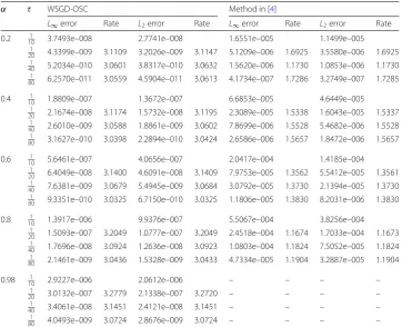
Table 7 TheL∞,L2errors and temporal convergence order withh= 1/1000 for Example4
α τ WSGD-OSC Method in [4]
L∞error Rate L2error Rate L∞error Rate L2error Rate
0.2 101 3.7493e–008 2.7741e–008 1.6551e–005 1.1499e–005
1
20 4.3399e–009 3.1109 3.2026e–009 3.1147 5.1209e–006 1.6925 3.5580e–006 1.6925 1
40 5.2034e–010 3.0601 3.8317e–010 3.0632 1.5620e–006 1.1730 1.0853e–006 1.1730 1
80 6.2570e–011 3.0559 4.5904e–011 3.0613 4.1734e–007 1.7286 3.2749e–007 1.7285
0.4 101 1.8809e–007 1.3672e–007 6.6853e–005 4.6449e–005
1
20 2.1674e–008 3.1174 1.5732e–008 3.1195 2.3089e–005 1.5338 1.6043e–005 1.5337 1
40 2.6010e–009 3.0588 1.8861e–009 3.0602 7.8699e–006 1.5528 5.4682e–006 1.5528 1
80 3.1627e–010 3.0398 2.2894e–010 3.0424 2.6586e–006 1.5657 1.8472e–006 1.5657
0.6 101 5.6461e–007 4.0656e–007 2.0417e–004 1.4185e–004
1
20 6.4049e–008 3.1400 4.6091e–008 3.1409 7.9753e–005 1.3562 5.5412e–005 1.3561 1
40 7.6381e–009 3.0679 5.4945e–009 3.0684 3.0792e–005 1.3730 2.1394e–005 1.3730 1
80 9.3351e–010 3.0325 6.7150e–010 3.0325 1.1806e–005 1.3830 8.2031e–006 1.3830
0.8 1
10 1.3917e–006 9.9376e–007 5.5067e–004 3.8256e–004
1
20 1.5093e–007 3.2049 1.0777e–007 3.2049 2.4518e–004 1.1674 1.7033e–004 1.1673 1
40 1.7696e–008 3.0924 1.2636e–008 3.0923 1.0803e–004 1.1824 7.5052e–005 1.1824 1
80 2.1461e–009 3.0436 1.5328e–009 3.0433 4.7334e–005 1.1904 3.2887e–005 1.1904
0.98 101 2.9227e–006 2.0612e–006 – – – –
1
20 3.0132e–007 3.2779 2.1338e–007 3.2720 – – – –
1
40 3.4061e–008 3.1451 2.4121e–008 3.1451 – – – –
1
80 4.0493e–009 3.0724 2.8676e–009 3.0724 – – – –
α∈(0, 1) and the last four columns present the numerical results obtained in [4]. From Table7, we find that the proposed method shows better performance than that in [4] for this example, since we adopt a higher-order approximation for the time derivative. In or-der to investigate the spatial convergence rate, we chooseτ= 1/1000 and list theL∞and
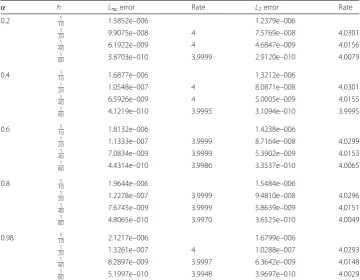
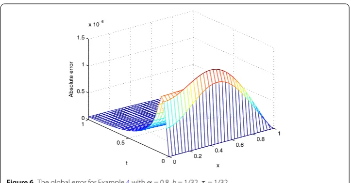
L2errors and corresponding convergence orders in Table8. Once again, the expected con-vergence rates with third-order accuracy in the time direction and fourth-order accuracy in the spatial direction can be seen from two tables. Besides, Fig.5shows a comparison of the numerical solution and the exact solution forα= 0.8 att= 1. The numerical solution surface is shown in Fig.6, and the errors are also displayed in Fig.7, whereα= 0.8 and
Table 8 TheL∞,L2errors and spatial convergence orders withτ= 1/1000 for Example4
α h L∞error Rate L2error Rate
0.2 101 1.5852e–006 1.2379e–006
1
20 9.9075e–008 4 7.5769e–008 4.0301
1
40 6.1922e–009 4 4.6847e–009 4.0156
1
80 3.8703e–010 3.9999 2.9120e–010 4.0079
0.4 1
10 1.6877e–006 1.3212e–006
1
20 1.0548e–007 4 8.0871e–008 4.0301
1
40 6.5926e–009 4 5.0005e–009 4.0155
1
80 4.1219e–010 3.9995 3.1094e–010 3.9995
0.6 101 1.8132e–006 1.4238e–006
1
20 1.1333e–007 3.9999 8.7164e–008 4.0299
1
40 7.0834e–009 3.9999 5.3902e–009 4.0153
1
80 4.4314e–010 3.9986 3.3537e–010 4.0065
0.8 101 1.9644e–006 1.5484e–006
1
20 1.2278e–007 3.9999 9.4810e–008 4.0296
1
40 7.6745e–009 3.9999 5.8639e–009 4.0151
1
80 4.8065e–010 3.9970 3.6525e–010 4.0049
0.98 1
10 2.1217e–006 1.6799e–006
1
20 1.3261e–007 4 1.0288e–007 4.0293
1
40 8.2897e–009 3.9997 6.3642e–009 4.0148
1
80 5.1997e–010 3.9948 3.9697e–010 4.0029
Figure 5The comparison (a) and absolute error (b) between the numerical solution and the exact solution withα= 0.8 att= 1 (h= 1/32,τ= 1/32)
7 Conclusion
Figure 6The global error for Example4withα= 0.8,h= 1/32,τ= 1/32
Figure 7Exact solution (a) and numerical solution (b) for Example4withα= 0.8,h= 1/32,τ= 1/32
Acknowledgements
The authors would like to thank the editor and referees for their valuable comments and suggestions for improving this manuscript significantly.
Funding
This work was supported by the National Natural Science Foundation of China (Grant Nos. 11601076, 11671131) and the Science and Technology Project of Jiangxi Provincial Education Department (Grant No. GJJ170473).
Competing interests
The authors declare they have no competing interests.
Authors’ contributions
All authors contributed equally and significantly in writing this paper. All authors read and approved the final manuscript.
Author details
1College of Mathematics and Statistics, Hunan Normal University, Changsha, P.R. China.2School of Science, East China
University of Technology, Nanchang, P.R. China.
Publisher’s Note
Springer Nature remains neutral with regard to jurisdictional claims in published maps and institutional affiliations.
Received: 3 November 2018 Accepted: 13 February 2019 References
1. Seki, K., Wojcik, M., Tachiya, M.: Fractional reaction–diffusion equation. J. Chem. Phys.119(4), 2165–2170 (2003) 2. Henry, B.I., Wearne, S.L.: Fractional reaction–diffusion. Physica A276, 448–455 (2000)
3. Sepehrian, B., Jabbari, M.: An implicit compact finite difference method for the fractional reaction–subdiffusion equation. Int. J. Appl. Math. Res.3(4), 579–586 (2014)
5. Chen, Y., Chen, C.M.: Numerical simulation with high order accuracy for the time fractional reaction–subdiffusion equation. Math. Comput. Simul.140, 125–138 (2017)
6. Jiang, Y., Ma, J.: High-order finite element methods for time-fractional partial differential equations. J. Comput. Appl. Math.235(11), 3285–3290 (2011)
7. Feng, L.B., Zhuang, P., Liu, F., Gu, Y.: Finite element method for space–time fractional diffusion equation. Numer. Algorithms72(3), 749–767 (2016)
8. Lin, Y.M., Xu, C.J.: Finite difference/spectral approximations for the time-fractional diffusion equation. J. Comput. Phys.
225(2), 1533–1552 (2007)
9. Liu, H., Lü, S.J., Chen, H., Chen, W.P.: Gauss–Lobatto–Legendre–Birkhoff pseudospectral scheme for the time fractional reaction–diffusion equation with Neumann boundary conditions. Int. J. Comput. Math. (2018).
https://doi.org/10.1080/00207160.2018.1450502
10. Dehghan, M., Abbaszadeh, M., Mohebbi, A.: Error estimate for the numerical solution of fractional reaction–subdiffusion process based on a meshless method. J. Comput. Appl. Math.280, 14–36 (2015)
11. Abbaszadeh, M., Dehghan, M.: A meshless numerical procedure for solving fractional reaction subdiffusion model via a new combination of alternating direction implicit (ADI) approach and interpolating element free Galerkin (EFG) method. Comput. Math. Appl.70, 2493–2512 (2015)
12. Dehghan, M., Manafian, J., Saadatmandi, A.: Solving nonlinear fractional partial differential equations using the homotopy analysis method. Numer. Methods Partial Differ. Equ.26(2), 448–479 (2010)
13. Saadatmandi, A., Dehghan, M.: A new operational matrix for solving fractional-order differential equations. Comput. Math. Appl.59(3), 1326–1336 (2010)
14. Ding, H., Li, C.: Mixed spline function method for reaction–subdiffusion equations. J. Comput. Phys.242, 103–123 (2013)
15. Li, X., Wong, P.J.Y.: A higher order non-polynomial spline method for fractional sub-diffusion problem. J. Comput. Phys.328, 46–65 (2017)
16. Yaseen, M., Abbas, M., Ismail, A.I., Nazir, T.: A cubic trigonometric B-spline collocation approach for the fractional sub-diffusion equations. Appl. Math. Comput.293, 311–319 (2017)
17. Huang, H., Cao, X.: Numerical method for two dimensional fractional reaction–subdiffusion equation. Eur. Phys. J. Spec. Top.222(8), 1961–1973 (2013)
18. Yu, B., Jiang, X.Y., Xu, H.: A novel compact numerical method for solving the two-dimensional non-linear fractional reaction–subdiffusion equation. Numer. Algorithms68, 923–950 (2015)
19. Yang, X., Zhang, H., Xu, D.: Orthogonal spline collocation method for the two-dimensional fractional sub-diffusion equation. J. Comput. Phys.256, 824–837 (2014)
20. Oruc, Ö., Esen, A., Bulut, F.: A Haar wavelet approximation for two-dimensional time fractional reaction–subdiffusion equation. Eng. Comput. (2018).https://doi.org/10.1007/s00366-018-0584-8
21. Li, X., Wong, P.J.Y.: Parametric quintic spline approach for two-dimensional fractional sub-diffusion equation. AIP Conf. Proc.1978(1), 130007 (2018).https://doi.org/10.1063/1.5043780
22. Dehghan, M., Safarpoor, M.: The dual reciprocity boundary elements method for the linear and nonlinear two-dimensional time-fractional partial differential equations. Math. Methods Appl. Sci.39(14), 3979–3995 (2016) 23. Bhrawy, A.H., Zaky, M.A.: A method based on the Jacobi tau approximation for solving multi-term time–space
fractional partial differential equations. J. Comput. Phys.281, 876–895 (2015)
24. Bhrawy, A.H., Zaky, M.A.: An improved collocation method for multi-dimensional space–time variable-order fractional Schrödinger equations. Appl. Numer. Math.111, 197–218 (2017)
25. Bhrawy, A.H., Zaky, M.A., Tenreiro Machado, J.A.: Legendre spectral tau algorithm for solving the two-sided space–time Caputo fractional advection-dispersion equation. J. Vib. Control22(8), 2053–2068 (2016)
26. Zaky, M.A.: An improved tau method for the multi-dimensional fractional Rayleigh–Stokes problem for a heated generalized second grade fluid. Comput. Math. Appl.75(7), 2243–2258 (2018)
27. Bhrawy, A.H., Zaky, M.A.: Numerical simulation of multi-dimensional distributed-order generalized Schrödinger equations. Nonlinear Dyn.89(2), 1415–1432 (2017)
28. Tian, W.Y., Zhou, H., Deng, W.: A class of second order difference approximations for solving space fractional diffusion equations. Math. Comput.84(294), 1703–1727 (2015)
29. Wang, Z., Vong, S.: Compact difference schemes for the modified anomalous fractional sub-diffusion equation and the fractional diffusion-wave equation. J. Comput. Phys.277, 1–15 (2014)
30. Ji, C.C., Sun, Z.Z.: A high-order compact finite difference scheme for the fractional sub-diffusion equation. J. Sci. Comput.64(3), 959–985 (2015)
31. Liu, Y., Zhang, M., Li, H., Li, J.C.: High-order local discontinuous Galerkin method combined with WSGD-approximation for a fractional subdiffusion equation. Comput. Math. Appl.73(6), 1298–1314 (2017)
32. Liu, Y., Du, Y.W., Li, H., Wang, J.F.: A two-grid finite element approximation for a nonlinear time-fractional cable equation. Nonlinear Dyn.85(4), 2535–2548 (2016)
33. Yang, X., Zhang, H., Xu, D.: WSGD-OSC scheme for two-dimensional distributed order fractional reaction–diffusion equation. J. Sci. Comput.76(3), 1502–1520 (2018)
34. Greenwell-Yanik, C.E., Fairweather, G.: Analyses of spline collocation methods for parabolic and hyperbolic problems in two space variables. SIAM J. Numer. Anal.23, 282–296 (1986)
35. Bialecki, B., Fairweather, G.: Orthogonal spline collocation methods for partial differential equations. J. Comput. Appl. Math.7, 55–82 (2001)
36. Li, C., Zhao, T., Deng, W., Wu, Y.J.: Orthogonal spline collocation methods for the subdiffusion equation. J. Comput. Appl. Math.255, 517–528 (2014)
37. Qiao, L., Xu, D.: Orthogonal spline collocation scheme for the multi-term time-fractional diffusion equation. Int. J. Comput. Math.95(8), 1478–1493 (2018)
38. Zhang, H., Yang, X., Xu, D.: A high-order numerical method for solving the 2D fourth-order reaction–diffusion equation. Numer. Algorithms (2018).https://doi.org/10.1007/s11075-018-0509-z
40. Jin, B., Lazarov, R., Liu, Y., Zhou, Z.: The Galerkin finite element method for a multi-term time-fractional diffusion equation. J. Comput. Phys.281, 825–843 (2015)
41. Fairweather, G., Gladwell, I.: Algorithms for almost block diagonal linear systems. SIAM Rev.46(1), 49–58 (2004) 42. Pani, A.K., Fairweather, G., Fernandes, R.I.: ADI orthogonal spline collocation methods for parabolic partial
integro-differential equations. IMA J. Numer. Anal.30(1), 248–276 (2010)
43. Robinson, M.P., Fairweather, G.: Orthogonal spline collocation methods for Schrödinger-type equations in one space variable. Numer. Math.68(3), 355–376 (1994)
44. Li, B., Fairweather, G., Bialecki, B.: Discrete-time orthogonal spline collocation methods for Schrödinger equations in two space variables. SIAM J. Numer. Anal.35(2), 453–477 (1998)
45. Meerschaert, M.M., Tadjeran, C.: Finite difference approximations for fractional advection-dispersion flow equations. J. Comput. Appl. Math.172(1), 65–77 (2004)
46. Percell, P., Wheeler, M.F.: AC1finite element collocation method for elliptic equations. SIAM J. Numer. Anal.17(5),
605–622 (1980)
47. Lin, Y.P., Thomee, V., Wahlbin, L.B.: Ritz–Volterra projections to finite-element spaces and applications to integrodifferential and related equations. SIAM J. Numer. Anal.28(4), 1047–1070 (1991)
48. Sun, W.: Block iterative algorithms for solving Hermite bicubic collocation equations. SIAM J. Numer. Anal.33(2), 589–601 (1996)