Spatial cross correlation modeling for propagation channels in indoor distributed antenna systems

(1)

R E S E A R C H

Open Access

Spatial cross-correlation modeling for

propagation channels in indoor distributed

antenna systems

Li Tian, Xuefeng Yin

*

, Xu Zhou and Quan Zuo

Abstract

In this contribution, the spatial cross-correlation of composite channels in a distributed antenna system (DAS) is studied for the case that a nine-antenna DAS is deployed in an indoor environment. As few measurement data of DAS propagation channels are available, the propagation graph modeling based on the electromagnetic wave

reverberation theory is used to generate the synthetic impulse responses (IRs) for the composite channels induced by the different groups of antennas in the DAS. The simulations take into account the geographic parameters of the environment, the cluttering scatterers, the realistic visibility conditions, as well as the flexible locations for the antennas, and the user equipment. The uncorrelated scattering assumption is proved to be valid by using the real measurement data from the indoor environments. Based on this assumption, narrowband channel cross-correlation is computed by integrating the small-scale fading cross-correlation within the same delay bins in two channel IRs. The characteristics of the cross-correlation in four cases with different antenna grouping are investigated for the

nine-antenna DAS. Part of the modeling results are shown to be consistent with the empirical counterparts for specific DAS constellations calculated using the real measurement data.

1 Introduction

A distributed antenna system (DAS) is referred to as the network of spatially separated antenna nodes con-nected to a common access point. The DAS has several advantages, comparing with the traditional concentrated multiple-input-multiple-output (MIMO) system (CMS). First, it allows the same coverage of an area with less power consumption since the distributed antennas cre-ate line-of-sight (LoS) connections to the mobile station, which can significantly reduce the power consumption caused by wall penetration inside buildings. Also, it reduces the delay spreads of the received signals, as well as the complexity of receivers [1,2]. The locations of anten-nas can be designed following different principles, e.g., achieving better coverage, enhancing spectral efficiency [3], or increasing the quality of received signals [4].

Recently, the transmission technologies for DAS have attracted a lot of attention [5,6]. For example, in [5], block diagonalization and zero-forcing dirty-paper coding

*Correspondence: [email protected]

College of Electronics and Information Engineering, Tongji University, Shanghai, China

downlink transmission schemes are extended for a single-cell DAS with multi-antenna-distributed antenna nodes. Only a subset of the antenna nodes in the cell transmits to the user equipment (UE). The aggregate cell spectral effi-ciency achieved by the proposed schemes per frequency-time resource block is compared for both DAS and CMS architectures. It has been demonstrated that, under the same total power constraint, the cellular DAS can double the ergodic aggregate cell spectral efficiency of the CMS. In addition, the spectral efficiency increases and saturates as the number of antennas per node increases. In [6], a generalized DAS combined with the CMS is introduced, where each distributed node has multiple micro-diversity antennas. All the antennas have a separate feeder to the base station. The signals can be combined using different algorithms.

For the existing theoretical studies of DAS, oversimpli-fied propagation channel models and ideal assumptions are usually adopted for the performance analysis [6]. The impact of real environment on the DAS performance has not been thoroughly investigated. In these simplified channel models, the power of a single channel at each

(2)

antenna in a distributed antenna node follows the chi-squared distribution with two degrees of freedom (χ₂2), while the mean of the distribution varies independently with log-normal distribution. The average of stochastic power means of the antennas within a node is determined by the path loss from the UE to the node, neglecting the shadow fading attributed to the UE surroundings. The ‘inter-node’ and the ‘intra-node’ fadings are assumed to be independent and identical log-normal and Rayleigh distri-butions, respectively. According to [6], the independence of the ‘inter-node’ fading is justifiable by the large distance between any two nodes and the distinctive scattering around the antennas in each node. However, as illustrated in [7], propagation environments, particularly the indoor propagation environment, introduce significant depen-dence among the nodes even when these aforementioned conditions are satisfied. Therefore, field measurements or realistic simulations are essential for establishing DAS channel models in both macroscopic and microscopic view points.

In this contribution, a simulation approach is applied to analyzing the characteristics of fading correlation across multiple links in DAS scenarios. The electromagnetic (EM) wave reverberation theory, originally adopted in [8] for generating channel impulse response (IR), is adopted to create the synthetic IRs in DAS scenarios. The spa-tial cross-correlations are then investigated by taking into account specific DAS configurations in an indoor envi-ronment. The validity of the predicted characteristics is evaluated using measurement data.

The organization of this paper is as follows: section 1 gives the general background of the works; in section 2, the approach of DAS channel simulations based on prop-agation graph are elaborated, and the simulations are validated using measurement data; in section 3, the spa-tial cross-correlation for DAS channels is defined; the simulation results for an indoor scenario are presented in section 4; experimental confirmation of the char-acteristics predicted by the simulations is depicted in section 5; finally, conclusive remarks are addressed in section 6.

2 Propagation graph modeling for DAS channels

2.1 A brief introduction of graph modeling

The propagation graph modeling approach has been applied to predicting channel IRs in [8] by exhaus-tively searching of the propagation paths connecting the transmitters and receivers. A propagation graph can be generated by taking into account the geometry of the envi-ronment, the scatterers’ distribution, the mobility, and visibility of the scatterers, as well as the scatterers’ EM properties.

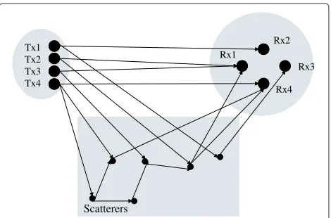
For example, as shown in Figure 1, if the position and visibility information of transceivers and scatterers has

Tx1

Figure 1An example of propagation graph with four transmitters (Tx), four receivers (Rx), and six scatterers.

been configured, the transfer function of the propagation can be calculated in the frequency domain as [8]:

H(f)=D(f)+R(f)[1+B(f)+B2(f)

+ · · · +Bn₍_f₎_{+ · · ·}_]_T₍_f₎

=D(f)+R(f)[1−B(f)]−1T(f), (1) where D(f) represents the LoS part of the transmis-sion, and R(f)[1 − B(f)]−1_T₍_f₎ _{is the none}

line-of-sight (NLoS) component induced by the reverberation of EM waves among scatterers. In Equation 1, T(f), R(f), and B(f) denote the transmission matrices with entries representing the power attenuations and phase changes from individual transmitter (Tx) to scatterers, from scatterers to individual receiver (Rx), and among scatterers, respectively. Bn(f) refers to the nth bounce inter-reflections of the scatterers. The transfer function of a propagation path that represents a link in Figure 1 can be calculated as:

Ae(f)=ge(f)exp(j2πτef +jφ), (2)

where Ae is an element in the matrics D, T, B, and R

according to different kinds of link ends, ge(f) is the

propagation coefficient calculated based on the free-space propagation loss and the reflection coefficient, τe is the

delay or time of arrival, andφ is the random phase rota-tion, which follows a uniform distribution on the interval [0, 2π).

(3)

Figure 2The 3D diagram of the building for an indoor environment considered.

100 scatterers in a snapshot costs about 8×106flops which can be executed in less than 0.1s using the computing software, e.g., MATLAB˝owith a quad-core computer. In addition, the IR obtained by the graph approach exhibits the specular-to-diffuse transition, which is hard to obtain using conventional ray-tracing-based channel modeling with tractable complexity [9-11].

The effectiveness of applying the graph approach to channel modeling has been investigated in [8] and [12], where the power-delay profiles and the specular-to-diffuse transition of the simulated IRs are compared with

those of the real IRs. In [13], the spatial and temporal characteristics of the channel IRs generated by graph in high-speed railway scenarios have been shown to be real-istic. In this contribution, the graph modeling approach is further evaluated in an indoor scenario by comparing the statistical characteristics of channel parameters obtained from graph modeling with the parameter values specified in established WINNER II channel models [14]. It will be shown later in section 2.2 that the typical channel char-acteristics predicted by the graph modeling is consistent with the WINNER II models.

2.2 Evaluation of propagation graph modeling

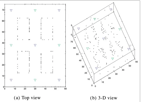
An indoor hall environment as depicted in Figure 2 is con-sidered for evaluating the applicability of graph-modeling in reproducing realistic channel characteristics. The hall is 60-m wide, 70-m long, and 5-m high. Within the hall, a number of rectangular structures exist, which attenuate the EM waves dramatically and have significant impact on the visibility among the scatterers and the antennas. In total, nine distributed antennas are deployed in the hall. The locations of the antennas are marked with ‘∇’

0

0 1100 2200 3300 4400 5500 6600 0

0 1 100 2 200 3 300 4 400 5 500 6 600 7 700

0 0

1 100

2 200

3 300

4 400

5 500

6 600

0 0 1 100 2 200 3 300 4 400 5 500 6 600 7 700

0 0 5 5

(( ))

aa T

To

op

p v

viieew

w

(( ))

b

b 3

3--D

D v

viieew

w

(4)

in Figure 3a. Scatterers are randomly distributed either on the inner walls of the hall or on the outer walls of the inside structures (See Figure 3b for the locations of the scatter-ers) to emulate the multi-reflection and diffuse scattering. There are also some scatterers located at the corners of the walls to emulate the diffraction. The parameters used in the graph modeling approach are listed in Table 1.

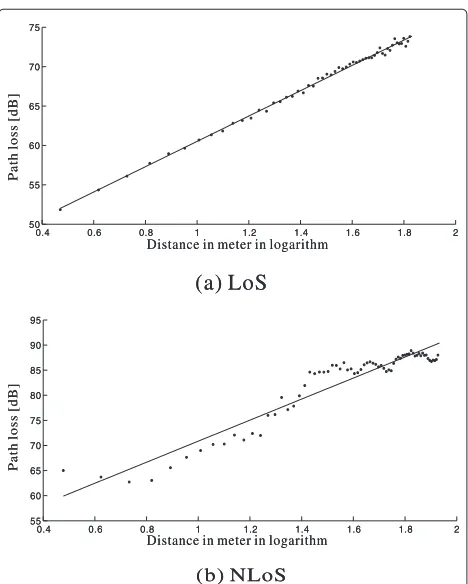
This indoor environment can be categorized as the optional A1 scenario specified in WINNER II SCM mod-els [14]. To evaluate modeling accuracy using propagation graphs, two large-scale channel parameters, i.e., path loss and delay spread are chosen for comparison between the graph models and the standard WINNER II mod-els. Totally, 12, 384 IRs are generated using the propa-gation graphs for 1, 376 UE locations, i.e., nine graphs per UE location. According to the visibility between the UE and the antennas, the IRs are split into the LoS group and the NLoS group. The path losses and delay spreads are computed for the two groups separately. Figure 4a,b depict the path loss versus distance in base-10 logarithm of meters for LoS and NLoS, respectively. The regression lines fitted to the simulated samples are also illustrated. It can be observed that the slope of the line equals 16 for LoS and 20.96 for NLoS. According to the WINNER II models, this parameter equals 18.7 for LoS and 20 for NLoS (see p. 44 in [14]). There-fore, we consider that the results obtained with graph models are sufficiently close to the standardized model parameters.

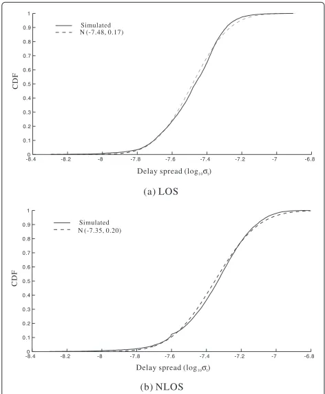
Figure 5 depicts the cumulative distribution functions (CDFs) of the delay spreads calculated, respectively, from the individual snapshots of the LoS and NLoS scenarios generated by the graph models. It can be seen that the delay spreads in logarithm can be well characterized by Gaussian distributions, the means and variances are

Table 1 Parameter settings for graph-based IR simulations

Description Value

Carrier frequency 2.6 GHz

Bandwidth 20 MHz

Heights of Tx antennas 4.6 m

Height of scatterers [0, 5] m

Heights of UEs 1.7 m

Total UE locations 1, 376

Snapshots per location 150

Signal to noise ratio 30 dB

Number of Tx antennas 9

Number of UE antennas 1

Groups of Tx antennas 2

Reflection gain 0.8

Figure 4Path loss of channels simulated in indoor LoS (a) and NLoS (b) environment.Regression lineP=16.08 log10d+44.45 is used to fit the results in LoS, andP=20.96 log10d+49.90 is used to fit the results in NLoS.

also quite close to the standard values presented in the WINNER II models (see p. 47 in [14]).

(5)

- .08 4 - .8 2 -8 - .7 8 - .7 6 - .7 4 - .7 2 -7 - .6 8

Figure 5Delay spreads in logarithm for channels simulated in indoor LoS (a) and NLoS (b) environment respectively.

predicted by properly tuning the parameters of the graph models.

3 Definition of spatial fading cross-correlation

The spatial fading cross-correlation coefficient ρ is defined as the cross-correlation coefficients of the

Figure 6Mean of delay spread in logarithm versus reflection gain in indoor scenario.

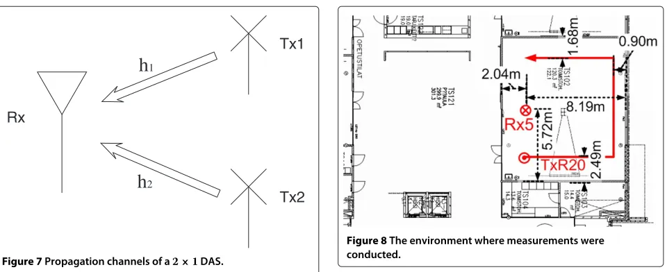
narrowbanda fading of links ‘1’ and ‘2’ observed at the same UE location, i.e.,

ρ= E[(h1− ¯h1)(h2− ¯h2)∗]

whereh1andh2denote the complex narrowband channel

coefficients of two links, respectively, as shown in Figure 7 andh¯is the mean of the channel coefficient.E{·}denotes the expectation operation. Defining the mean-removed channel coefficientshˆ1 =h1− ¯h1andhˆ2 = h2− ¯h2, the

whereh(τ)denotes the complex-valued spread function of the channel in delay andTis the observing time of each snapshot.

From Equation 4, it is clear thatC1,2 is split into two

parts, i.e., the common-delay (cmd) part and cross-delay (crd) part. The narrowband fading cross-correlation coef-ficientρcan then be written as:

ρ= C1,2

where the discrete equivalents of cross-correlation coeffi-cients of the cmd componentsρcmdand crd components ρcrdcalculated in reality are expressed as:

(6)

Tx1

Tx2

Rx

h

1

h

2

Figure 7Propagation channels of a2×1DAS.

respectively, whereIis the number of the channel coeffi-cient samples in each UE location andNis the number of delay samples in each complex-valued spread function of the channel.

In the case where the uncorrelated scattering (US) assumption is valid, the equality ρcrd = 0 holds as

the components with different delays are uncorrelated. However, in graph modeling, the cross-correlation among the different delay components is non-negligible because of the limited number of scatterers in the graphs. This implies that if we computeρby the channel coefficientsh1

andh2generated by graph modeling, wrong estimates may

arise sinceρcrd = 0 for the channels constructed by the

graphs. Alternatively, we consider to approximate theρby calculatingρcmdonly. The accuracy of this approximation

is evaluated in section 3.1 using measurement data.

3.1 Validation of the approximationρ≈ρcmd

The measurement data collected by the wideband channel sounder -PROPSound- in an office building in Oulu University, Finland [15] is considered for the evalua-tion of ρ ≈ ρcmd. Figure 8 depicts the map of the

measurement environment. During the measurements, the receiver was fixed, and the transmitter was mov-ing along the measurement route marked in red. The measured data were collected in cycles. Here, a cycle is the time duration that the channels between any pair of the transmitter antenna and the receiver antenna are measured once. The channel coefficients obtained in a measurement cycle can be considered as random obser-vations of the same wide-sense-stationary channel, due to the following reasons: (1) the radiation patterns of the antenna elements are nonidentical; (2) the system responses contain random phase noises when using any pair of Tx and Rx antennas; and (3) the channel is not exactly constant during the measurements, as slight

Figure 8The environment where measurements were conducted.

differences in small scale such as the movement of the person pushing the Tx trolley and the absorption give rise to the randomness in the observations of the chan-nel. Since the transmitter and the receiver were equipped with 50 and 32 antennas, respectively, for each cycle in total, 50×32= 1, 600 channel coefficients are obtained. These channel observations are used to calculate the fad-ing correlation coefficients. Figure 9 illustrates the con-tour plots of ρandρcmd computed based on the data of

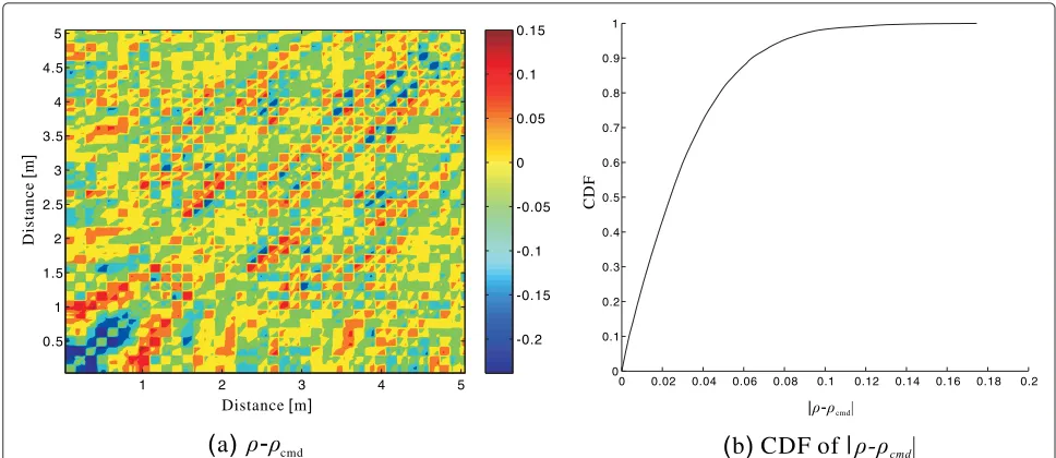
150 cycles, while the contour plot and the CDF of the devi-ations between ρ andρcmd are depicted in Figure 10. It

can be observed that most of the deviations betweenρand

ρcmdare close to zero. More than 97% of the deviations are

less than 0.1, and the mean value ofρ-ρcmdis about 0.02.

Thus,|ρ ≈ ρcmd|can be considered empirically valid in

indoor environments.

4 Modeling spatial cross-correlation of fading in a DAS

(7)

Figure 9Contour plot of the experimental cross-correlation coefficients.(a)depicts the coefficients of narrowband channels, and(b)depicts the coefficients of wideband common-delay components in IRs.

this position withinλ/4. This vicinity range is determined accordingly such that random realizations are in the same WSS condition. Then the fading correlation is calculated based on the simulated IRs.

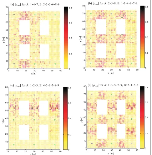
Figure 11 depicts the absolute values of fading cross-correlation observed at the UE when the composite chan-nels are generated using four different grouping schemes. In each scheme, groups A and B of antennas are spec-ified. We use ‘A:1−2 −3’ to denote that the group A consists of the antennas 1, 2, and 3. It can be observed

that the fading cross-correlation exhibits symmetric pat-tern in accordance with the antenna constellations as well as the geometry of the environment. Significant spa-tial cross-correlation can be observed at locations where groups A and B antennas are distributed symmetrically. This is reasonable as the propagation channels observed by the UE from two nearest antennas, which are both in the LoS positions to the UE, are very similar, e.g., as in the case where the UE is in the middle of two anten-nas which belong to different groups. Low spatial fading

Distance m[ ]

Distance

m

[]

( )

a

_cmd

1 2 3 4 5

0.5 1 1.5 2 2.5 3 3.5 4 4.5 5

- .0 2 - .0 15 - .0 1 - .0 05 0 0.05 0.1 0.15

0 0.02 0.04 0.06 0.08 0.1 0.12 0.14 0.16 0.18 0.2 0

0.1 0.2 0.3 0.4 0.5 0.6 0.7 0.8 0.9 1

CD

F

( )

b CDF of

|

(8)

Figure 11Spatial cross-correlation coefficients of composite channels in a DAS.Results of four-antenna grouping schemes are illustrated in the four subfigures(a,b,c,d).

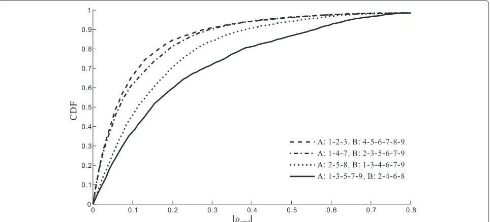
cross-correlation is observed at the locations where the groups A and B antennas are asymmetric with respect to (w.r.t.) the UE, e.g., when UE is located in the vicin-ity of the antennas. These observations hold for all four constellations illustrated in Figure 11. The CDFs of the fading cross-correlation coefficients in the four schemes are depicted in Figure 12. It can be observed that the con-figuration with locations of antennas in different groups

overlapped gives the highest cross-correlation coeffi-cients. When antennas belonging to different groups are separated, the cross-correlation becomes less.

(9)

Figure 12Cumulative distribution function of spatial cross-correlation coefficients of different groups in simulated DAS.

fading correlation in the environments of interest. A common belief for achieving better coverage and low-power consumption is to allocate antenna symmetri-cally for the DAS [1,2,16]y. However, the investigation results illustrated here show that the improvement by utilizing the DAS is marginal due to the non-negligible cross-correlation attributed to the symmetric antenna constellations.

5 Experimental evaluation

The spatial correlation in most of the DASs can be ignored because the spacing of the antennas are much larger than the coherent distance. However, in section 4, the simula-tion results show that significant fading cross-correlasimula-tion can be observed in the case where two transmitting anten-nas are distributed in symmetric locations w.r.t. the UE. In this section, we use measurement data collected in the same campaign described in section 3.1 to validate this observation.

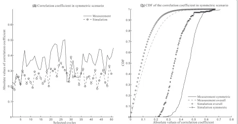
Figure 13 depicts a measurement environment where the locations of two distributed Txs are confined, respec-tively, in the two marked ranges that are symmetrical w.r.t. the Rx’s location along the dashed line. Furthermore, the environments surrounding the Txs are also symmetric w.r.t. the dashed line. In order to evaluate the conclusions drawn from the simulation results in section 4, multiple Tx pairs with image locations to the Rx are considered to construct 2×1 DASs. Knowing the exact cycle indices at the corner points, the IRs of 50 cycles collected in the marked regions are identified for these 2×1 DASs. Figure 14a illustrates the correlations of these selected cycles. It can be observed that both the measured and

simulated correlation coefficientsρare around 0.3 which are non-negligible in computing the diversity gain of the DAS.

In addition, the empirical statistics of the DAS chan-nel correlation are extracted based on the measurements. Figure 14b depicts the empirical and simulated CDFs of the absolute values of fading correlation coefficients for symmetric links only and all links. It can be observed from Figure 14b that 90% of the correlation coefficients for the measured symmetric links are larger than 0.3, while the

(10)

a b

Figure 14Fading correlation coefficients (a) and their CDFs (b) in specified DAS constellations.The solid line depicts the fading correlation of the links which poses the symmetric pattern, and the dash line represents the fading correlation of all the links based on measurement. Similarly, the symmetric and overall results based on simulation are depicted in squares and circles, respectively.

correlation coefficients of all links are much less and neg-ligible. Similar results are observed for the simulations, even though the correlation coefficients are underesti-mated in the simulations. It is our conjecture that the underestimation is due to the settings of random phase in Equation 2 for graph modeling approach which might not hold in realistic environment.

6 Conclusions

The spatial cross-correlation of channel fadings in dif-ferent links of a DAS has been investigated via sim-ulations using stochastic propagation graphs. We first proposed an approach for computing the fading cross-correlation, i.e., it is approximated by integrating the cross-correlation coefficients of the small-scale fadings in the same delay bins of two channels. The effectiveness of this approach has been evaluated using the measure-ment data. Then, the applicability of random propagation graphs in channel modeling was validated. It has been shown that the statistics of path loss and delay spreads extracted using graphs is close to those specified by the WINNER II models. Using the proposed methods, the narrowband fading cross-correlation of the composite channels in DASs for a hall-alike indoor environment has been investigated. The results obtained demonstrated that the highest cross-correlation coefficients can be observed when the locations of antennas in different groups are overlapped. When antennas belonging to different groups

are located in two well-separated regions, the cross-correlation becomes smaller. Moreover, significant fading cross-correlation can be observed in the cases where the distributed antennas belonging to different groups are deployed symmetrically w.r.t. the location of the UE. These results have been shown to be consistent with the observations obtained in real measurements.

Endnote

a_{Here, narrowband means that signal bandwidth times}

delay spread is much smaller than 1.

Competing interests

The authors declare that they have no competing interests.

Acknowledgments

(11)

Received: 20 September 2012 Accepted: 25 June 2013 Published: 8 July 2013

References

1. W Roh, High performance distributed antenna cellular networks. PhD thesis, Dept. Elect. Eng., Stanford Univ., Stanford, CA 2003.

2. H Xia, A Herrera, S Kim, F Rico, A CDMA-distributed antenna system for in-building personal communications services. IEEE J. Selected Areas Commun.14(4), 644–650 (1996). IEEE, Piscataway

3. T Alade, H Zhu, H Osman, inIEEE 22nd International Symposium on Personal Indoor and Mobile Radio Communications (PIMRC)Spectral efficiency analysis of distributed antenna system for in-building wireless communication (IEEE, Piscataway, 2011), pp. 2075–2079

4. J Lee, J Roh, J Kwun, C Kang, inIEEE International Conference on Universal Personal Communications (ICUPC), vol. 1 A controlled distributed antenna system for increasing capacity in the DS-CDMA system (IEEE, Piscataway, 1998), pp. 345–348

5. T Ahmad, S Al-Ahmadi, H Yanikomeroglu, G Boudreau, inIEEE 73rd Vehicular Technology Conference (VTC Spring)Downlink linear transmission schemes in a single-cell distributed antenna system with port selection (IEEE, Piscataway, 2011), pp. 1–5

6. W Roh, A Paulraj, inIEEE 56th Vehicular Technology Conference (VTC Fall), vol.3Outage performance of the distributed antenna systems in a composite fading channel (IEEE, Piscataway, 2002), pp. 1520–1524 7. X Zhou, X Yin, BJ Kwak, HK Chung, inProceedings of 5th European

Conference on Antennas and Propagation (EuCAP)Experimental

investigation of impact of antenna locations on the capacity of wideband distributed antenna systems in indoor environments (IEEE Piscataway, 2011), pp. 1639–1643

8. T Pedersen, B Fleury, inIEEE International Conference on Communications (ICC)Radio channel modelling using stochastic propagation graphs (IEEE Piscataway, 2007), pp. 2733–2738

9. T Fugen, J Maurer, T Kayser, W Wiesbeck, Capability of 3-D ray tracing for defining parameter sets for the specification of future mobile communications systems. IEEE Trans. Antennas Propagation.54(11), 3125–3137 (2006). IEEE, Piscataway

10. Y Lostanlen, G Gougeon, inInternational Conference on Electromagnetics in Advanced Applications (ICEAA)Introduction of diffuse scattering to enhance ray-tracing methods for the analysis of deterministic indoor UWB radio channels (Invited Paper) (IEEE Piscataway, 2007), pp. 903–906 11. V Degli-Esposti, D Guiducci, A de’Marsi, P Azzi, F Fuschini, An advanced

field prediction model including diffuse scattering. IEEE Transact. Antennas Propagation.52(7), 1717–1728 (2004). IEEE, Piscataway 12. T Pedersen, G Steinbock, BH Fleury, Modeling of reverberant radio

channels using propagation graphs. IEEE Trans. Antennas Propagation. 60(12), 5978–5988 (2012). IEEE, Piscataway

13. L Tian, X Yin, Q Zuo, J Zhou, Z Zhong, SX Lu, inIEEE 23rd International Symposium on Personal Indoor and Mobile Radio Communications (PIMRC) Channel modeling based on random propagation graphs for high speed railway scenarios (IEEE Piscataway, 2012), pp. 1746–1750

14. P Kyosti, J Meinila, L Hentila, X Zhao, T Jamsa, C Schneider, M Narandzic, M Milojevic, A Hong, Ylitalo J, V-M Holappa, M Alatossava, R Bultitude, Y de Jong, T Rautiainen, Winner II channel models (d1.1.2v1.1). (2007). http:// www.ist-winner.org/WINNER2-Deliverables/D1.1.2v1.1.pdf.

Accessed Nov 2007.

15. N Czink, The random-cluster model - a stochastic MIMO channel model for broadband wireless communication systems of the 3rd generation and beyond. PhD thesis, Technische Universitat Wien, Vienna, Austria, FTW Dissertation Series, 2007.

16. X Hu, Y Zhang, Y Jia, S Zhou, L Xiao, inFourth International Conference on Communications and Networking in China (ChinaCOM)Power coverage and fading characteristics of indoor distributed antenna systems (IEEE Piscataway, 2009), pp. 1–4

doi:10.1186/1687-1499-2013-183

Cite this article as:Tianet al.:Spatial cross-correlation modeling for

propa-gation channels in indoor distributed antenna systems.EURASIP Journal on

Wireless Communications and Networking20132013:183.