Volume 2008, Article ID 729180,8pages doi:10.1155/2008/729180
Research Article
Decoding LDPC Convolutional Codes on Markov Channels
Manohar Kashyap and Chris Winstead
Department of Electrical and Computer Engineering, College of Engineering, Utah State University, Logan, UT 84322-4120, USA
Correspondence should be addressed to Manohar Kashyap,[email protected]
Received 31 August 2007; Accepted 26 February 2008
Recommended by Yonghui Li
This paper describes a pipelined iterative technique for joint decoding and channel state estimation of LDPC convolutional codes over Markov channels. Example designs are presented for the Gilbert-Elliott discrete channel model. We also compare the performance and complexity of our algorithm against joint decoding and state estimation of conventional LDPC block codes. Complexity analysis reveals that our pipelined algorithm reduces the number of operations per time step compared to LDPC block codes, at the expense of increased memory and latency. This tradeoffis favorable for low-power applications.
Copyright © 2008 M. Kashyap and C. Winstead. This is an open access article distributed under the Creative Commons Attribution License, which permits unrestricted use, distribution, and reproduction in any medium, provided the original work is properly cited.
1. INTRODUCTION
LDPC convolutional codes (LDPC-CCs) are the convolu-tional counterparts of LDPC block codes (LDPC-BCs) and were first presented in 1999 by Feltstr¨om and Zigangirov [1]. Algorithms have been studied for decoding LDPC Convolutional codes over memoryless channels, such as the additive white Gaussian noise (AWGN) channel. LDPC-CC decoding over channels with memory has not been addressed to date. Wireless channels typically have memory, and are often approximated using discrete Markov channel models, of which the simplest is the well-known Gilbert-Elliott model.
LDPC-CC codes are attractive for three main reasons. First, they support arbitrary frame lengths, which is useful in packet-switched networks. Second, they achieve perfor-mance comparable to conventional LDPC codes. Finally, LDPC-CC decoders can be implemented using a pipelined architecture that significantly reduces the number of active operations required per iteration.
Markov models are widely used to represent time-varying communication channels [2]. If the channel is subject to significant variation within a transmitted frame, then performance can be significantly improved if decoding and channel state estimation are performed jointly using iterative algorithms.
This paper introduces a new algorithm for LDPC-CC decoding over Markov channels. The new algorithm applies the general principles of joint inference [3, 4] to
the specialized problem of efficient LDPC-CC decoding on channels with memory. We demonstrate that joint decoding and channel state estimation can be performed by adding a few steps to the pipeline decoding algorithm. This means that the cost of adding joint channel state estimation to an existing LDPC-CC decoder is extremely small. We show that when complexity is measured as arithmetic operations per iteration, joint state estimation and decoding is much less complex for LDPC-CCs than for traditional LDPC block codes. The tradeoffis that LDPC-CC decoders require con-siderably more memory, but in most cases this is a favorable trade in terms of power, complexity, and circuit area.
As a proof-of-concept demonstration, we apply our algo-rithm to joint decoding and state estimation on the Gilbert-Elliott channel. The Gilbert-Gilbert-Elliott channel [5] represents a burst-error channel which toggles between “good” and “bad” binary symmetric channel states. Interleaving methods were previously used to remove the memory from a Gilbert-Elliott channel, but this technique resulted in substantially reducing the channel’s effective capacity [6]. More recently, it was shown that joint state estimation and decoding of turbo codes on Gilbert-Elliott channels allows transmission at rates closer to the Gilbert-Elliott channel’s native capacity [7]. Our algorithm provides a power-efficient adaptation of these approaches for the LDPC-CC case.
Section 3.4presents the new pipelined estimation-decoding algorithm for LDPC-CCs. Section 4 presents performance and complexity analysis, for example, LDPC and LDPC-CC codes over the Gilbert-Elliott channel. Section 5offers conclusions.
The paper uses the following notation. Random variables and their quantities are indicated by lower-case Latin letters. IfXandY are random variables, then Pr{x | y}should be taken to mean the probability thatX=x, given thatY =y. Sets are indicated by upper-case Latin letters. Sequences are indicated by lower-case bold letters, and matrices by upper-case bold letters. Lower-upper-case Greek letters are used to indicate probability messages in the decoding algorithm.
2. LDPC CONVOLUTIONAL CODES
2.1. Code structure
LDPC-CCs are a family of time-varying convolutional codes with characteristics similar to conventional LDPC block codes (LDPC-BCs). LDPC-CCs are defined by a periodic low-density parity-check matrix:
whereM is the memoryandT is theperiodof the LDPC-CC, andt ∈ Zis the time index. The submatricesHTi(t+ i),i=0,. . .,Marec×(c−b) binary matrices, wherebis the number of information bits that enter the encoder, andcis the number of coded bits that exit the encoder at a given time index. The rate of the code isR=b/c. The memory is equal to the largestisuch thatHT
i(t+i) is a nonzero matrix, and T=M(c−b). An example parity-check matrix for anM=7 rate-1/2 LDPC-CC is shown inFigure 1.
Similar to the Tanner graph representation of LDPC-BCs, LDPC-CCs can also be represented graphically [8].Figure 2
shows a Tanner graph representation corresponding to the parity-check matrix inFigure 1. The Tanner graph exhibits a pattern that repeats itself (for time invariant LDPC-CCs) every M time indices or, equivalently, every Mc symbol nodes. Edges are present between symbols and check nodes when a “1” is present in the corresponding location of the parity-check matrix.
2.2. Decoding LDPC-CCs on memoryless channels
The seminal paper on LDPC-CCs [1] presented an iterative decoding strategy for memoryless channels. In this subsec-tion, we briefly review the LDPC sliding window decoding algorithm using factor graphs as in [8].
The LDPC-CC decoder is a chain of sliding window processors performing sum product algorithm (SPA) [9] calculations on symbols within the window. While an LDPC-BC decoder performs parallel operations on symbol and
1
Figure 1: An example parity-check matrix, HT, for a rate-1/2
LDPC-CC. The row indices correspond to symbols (i.e., channel bits), and the column indices correspond to parity check equations.
M
· · ·
Figure 2: Tanner graph corresponding toFigure 1. The circles indicate symbol nodes, and the squares indicate parity-check nodes.
parity-check nodes, iterations in the LDPC-CC decoder happen sequentially. As a symbol node shifts through the sliding window, SPA operations are performed on some of its edges. SPA operations are split into two phases per time index. During the verticalphase, SPA operations are performed on bparity-check nodes. During the horizontal phase, SPA operations are performed on c symbol nodes. The LDPC-CC H matrix is designed to guarantee that all necessary SPA operations are performed on a node afterM+1 time shifts, just before the symbol node exits the window [1]. For a rate-b/c(J,K) LDPC-CC decoder, the vertical and horizontal phases require Kb and Jc SPA operations, respectively.
To carry out multiple iterations, abutting sliding window processors are used. As a node exits one processor, it enters the next processor for an additional iteration. Therefore, for
Proc I Proc I-1 Proc 2 Proc 1
· · ·
Figure3: The LDPC-CC decoder sliding window represented as a series of processors.
1 1.5 2 2.5
Eb/N0
−6
−5
−4
−3
−2
−1 0
log
1
0
(BER)
M=128
M=512
M=2048
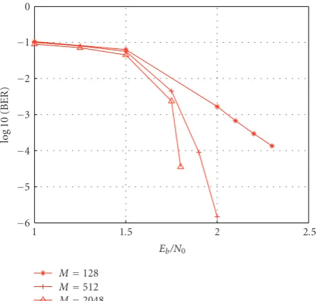
Figure4: LDPC-CC decoder performance over the AWGN channel, based on codes and algorithms from [10].
Figure 3shows the decoder window in operation over a rate
1/2 code, sliding from right to left.
The sliding window abstraction is very useful from a hardware design perspective. A designer only needs to implement one of these processors as a hardware block. The complete decoder is then constructed by tiling I copies of the processor block. As a point of reference, a comparison of the BER plots for rate 1/2 LDPC-CC and LDPC-BC codes on the AWGN channel [10] reveals that an M = 128 LDPC-CC has roughly the same performance as an
N=1024 LDPC-BC. InSection 4, we demonstrate that this rough equivalence also holds for joint decoding and state estimation on Gilbert-Elliott channels.Figure 4summarizes AWGN decoding results obtained in [10].
3. JOINT ESTIMATION DECODING
In this section, we present an iterative decoding algorithm for LDPC-CCs over channels with memory. Memory in channel states is modeled as aMarkov chain, hence the name Markov channel. We review the Gilbert-Elliott channel and LDPC-BC decoding over Markov channels before presenting the LDPC-CC decoding algorithm. All of these algorithms employ the SPA on factor graphs of the decoder. The general procedure followed in deriving these algorithms is as follows, summarized from [11]:
(1) derive the factor graph (or, equivalently, the Tanner graph) of the code constraints. The factor graph represents the probability mass function (PMF) of the code itself, as elaborated in [9]. In the typical case where all codewords are equiprobable, the code’s PMF is determined by thecharacteristic function:
Υ(x)= ⎧ ⎨ ⎩
1, x is a code word
0, otherwise. (2)
(2) Derive the conditional joint PMF of the received vectoryand the channel statess, that is, Pr(y,s|x). For discrete channels, the PMF takes the form of a Markov state-transition model, which has a well-known factor graph structure.
(3) The joint PMF describing the code and channel, Pr(y,s,x), is the product of the above derived PMFs, Υ(x) and Pr(y,s | x). The corresponding decoder factor graph is constructed by joining together the channel graph and the code graph at their intersect-ing symbol nodes.
3.1. Markov channels
A Markov channel is characterized by a set of states, S, which models the channel’s memory. At any time index i, the channel is in some statesi ∈ S. At each time index, the
channel’s state can undergo a random transition governed by the state transition probability matrixP. Letρibe the PMF
vector for the channel’s state at timei. Thenρi+1=P×ρi.
For a general Markov channel, the PMF of the channel state process can be written as
Pr(s)=Pr(s1)
n
i=1
Pr(si+1|si), (3)
where Pr(si+1 |si) are obtained fromP, the state transition
probability matrix of a general Markov channel. The channel state affects the channel output probability through a conditional PDF fyi(yi |xi,si) for eachsi ∈S. Letγibe the
channel informationwhich is conditional upon the channel state, defined as
γi(yi,xi,si,si+1)=Pr(si+1|si)fyi(yi|xi,si). (4)
In the sequel, the arguments to γi are be omitted, but γi should always be understood to have the functional
dependence as expressed by (4).
Then the conditional joint PMF of the received symbols and channel states is
Pr(y,s|x)=Pr(s1)
n
i=1
γi, (5)
3.2. Gilbert-Elliott channel
The Gilbert-Elliott (GE) channel [5] is a binary input-output Markov channel. It is a binary symmetric channel (BSC) whose inversion probability is modulated by a Markov chain. It can be described as
y=x⊕z, x,y,z∈ {0, 1}n
, (6)
wherex,y, andzare the channel input, the channel output, and the error sequence, respectively. The GE channel has two states, good and bad, as indicated in the channel model [5]. Each state contains a BSC with its own inversion probability. In the good state, the inversion probability is lower than the bad state. The error sequencezis a random sequence. At any given time, the error probability is
Pr(zi=1|si)=
whereηB andηG are the inversion probabilities in the bad
and good channel states, respectively.
If the good and bad states are assigned to numerical values 1 and 0, respectively, then the state transition matrix Pis
wherebandgare the 1→0 and 0→1 transition probabilities, respectively. The matrix elements arepjk=Pr(si+1=j|si= k). The last term needed to computeγiis the channel PDF:
fyi(yi|xi,si)=
3.3. LDPC BC decoding on Markov channels
Iteratively decoded codes allow for channel estimation during the decoding process and these estimates can further assist in decoding and vice versa. This is known asjoint esti-mation decoding. In this subsection, we review an estimation-decoding algorithm first presented in [6] and analyzed for LDPC-BCs in [3,4,11,12]. InSection 3.4, these concepts are adapted for use with LDPC-CCs.
To characterize the PMF of the channel, it is convenient to decompose the characteristic function,Υ(x), into compo-nent functionshj(x) representing the individual rows of the
parity-check matrix:
The joint PMF of the transmitted codeword received symbol sequence and channel states is then given by
Pr(y,s,x)=ξPr(s1)
Figure 5: Joint factor graph for decoding and channel state estimation of an LDPC-BC on a Markov channel [11].
whereξis the normalization constant forΥ(x), andN and
Mare the dimensions of the parity-check matrix.
The factor graph corresponding to (11) is shown in
Figure 5. The channel state and transition nodes comprising the Markov chain form the Markov subgraph. The symbol and check nodes of the classic LDPC graph form theLDPC subgraph. Joint state estimation and decoding are then performed by applying the SPA using a flooding schedule. In the LDPC subgraph, the ζ messages are substituted in place of the channel information. The χ messages are the a posteriori probabilities computed using the usual LDPC decoding computations.
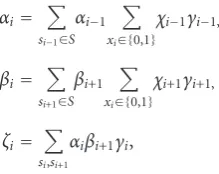
In the Markov subgraph, BCJR operations are performed with theχmessages applied as a priori information. At the start of each iteration, every node in the factor graph receives messages from adjacent nodes in the graph. Each message is a local conditional PMF. To complete the iteration, the SPA algorithm is applied to update the outgoing messages at each node in the graph. Theα,β, andζmessages have the usual definition, based on the BCJR algorithm, and are updated according to the standard rules:
αi= xi, and the function arguments are again omitted.
3.4. LDPC convolution decoding on Markov channels
To derive the decoder graph, we combine the Markov channel factor graph with the graph of an LDPC con-volutional code by joining the two graphs at the shared symbol nodes,xi. The derivation of the LDPC convolutional
code characteristic function, and hence its factor graph, is followed by the derivation of the decoder PMF, and hence the decoder graph, in the next few paragraphs.
The sequenceυ = (. . .,υ0,υ1,υ2,. . .),υt ∈ Fc2 forms a
convolutional code frame (equivalent to a block codeword) if and only if the constraint imposed by the syndrome former of the convolutional code is fulfilled, that is,
υtHT0(t) +υt−1HT1(t) +· · ·+υt−MHTM(t)=0. (13)
The characteristic function of the convolutional code is
Υ(υ)= ⎧ ⎨ ⎩
1, if (13) is satisfied for allt ∈Z,
0, otherwise. (14)
The convolutional characteristic function can be decom-posed as a product of component functions over time. Letxj
be defined as the sequence (υj,υj−1,. . .υj−M), corresponding
to the symbols in the encoder’s memory. Then at thejth time instant, the characteristic component function is
hj(xj)=
The convolutional characteristic function is then the product of the component functions over time:
Υ(υ)=
tend
j=0
hj(xj), (16)
wheretendis the time at which the convolutional sequence terminates.
To construct the joint PMF of the convolutional code and the Markov channel model, we note that there arecchannel symbols per time index in our notation, and therefore also
cMarkov channel states per time index. Let nbe the total number of channel symbols transmitted, that is,n=tend×c. Then,
The factor graph for the LDPC convolutional decoder is shown in Figure 6. Notice that the Markov channel graph
of Figure 5 has been wrapped around the convolutional
graph ofFigure 3resulting in a graph suitable for sequential operations. As the decoding window slides across this graph, it completes SPA operations oncchannel state variable nodes along withcsymbol nodes and (c−b) check nodes at each time index.
Joint decoding and estimation is performed using a flooding schedule as follows. Whenever a symbol node is updated in the decoder, the adjacent Markov state variables are also updated. At each time index in the LDPC-CC
si+4
Figure 6: Joint factor graph for an LDPC-CC decoder over a Markov channel. The Markov model wraps around the LDPC-CC factor graph.
pipeline, the χ messages are updated for c symbol nodes using the usual decoding operations. To perform the Markov state update, the α, β, and ζ messages are subsequently computed for each updated symbol node.
Whenever processing is completed for a node xi, the
resulting χi message is used to update αi, βi, and ζi. The
entire column of updated messages is then passed to the next processor, which performs the subsequent iteration. Messages on the Markov subgraph are updated directly alongside thexisymbol nodes within the pipeline.
Figure 7 shows the memory-based architecture for a
typical LDPC-CC processor, augmented to support joint channel state estimation [10,13,14]. Each column in the memory grid represents a symbol node. Each row represents a message passed along an edge in the code’s factor graph. Each symbol node is connected to the channel and to (up to)
Jparity-check nodes. Due to the structure of the LDPC-CC factor graph, a symbol’s influence vanishes afterM×ctime steps, so this is the number of columns that needs to be stored in the memory.
The processor requires one row to store channel informa-tion for each symbol andJ rows to store messages between variable and check nodes in the LDPC-CC subgraph. For a Markov channel withSstates, 2S+2 extra rows must be added to support channel state estimation. In the particular case of the GE channel, whereS =2, six extra rows are needed. SPA operations are completed forcsymbol nodes per time index per processor, so each processor needs to update 4c
additional messages per time index per processor to perform joint state estimation. As these messages pass through the pipeline of processors, updates propagate across the Markov subgraph.
3.5. Alternative message passing schedules
M×c
J
c
State-estimation operations
State-estimation
memory
Figure 7: The memory-based LDPC-CC decoding architecture
for a rate-1/2 code, highlighting the extramemory resources and additional operations needed to implement joint channel state estimation.
estimation/decoding, for example, is known to provide improved performance for LDPC block codes in some cases, but cannot obviously be applied to the LDPC-CC case.
In the turbo schedule, Markov state estimation is carried out using the BCJR algorithm on a sliding window. All
α, β, and ζ messages are computed while the χ messages are held constant. Meanwhile, the decoder computes newχ
messages by performing one iteration with the ζ messages held constant. This schedule requires thatblocks of symbol messages be exchanged between the estimator and the decoder. Because the pipelined decoder computes only c
symbol messages per time index, it is not possible to accumulate a large frame of messages without interrupting the pipeline.
4. PERFORMANCE RESULTS
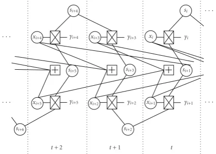
Figure 8 shows the BER plot for rate 1/2, (3, 6) LDPC
convolutional codes with memories 128, 256, and 2048 with channel parameters (b,g,ηG)=(0.01, 0.01, 0.01), whereηBis
swept from 0.04 to 0.18. As expected, decoding gain increases with memory. As with joint estimation and decoding on LDPC-BCs, LDPC-CCs are observed to have low error floors.
Figure 9plots the BERs for anM=128 code, with iterations ranging from 10 to 60. Statistically, significant improvements are not observed for pipelines longer than 50 processors.
4.1. Comparison of LDPC-BC and LDPC-CC decoders
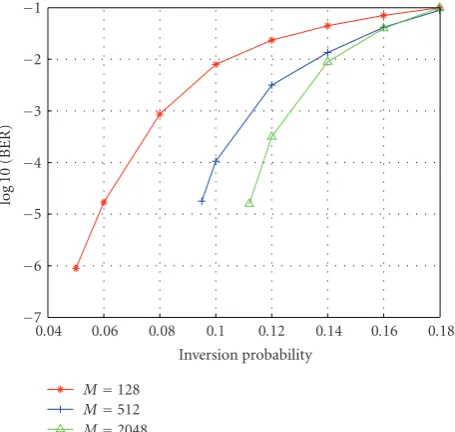
Figure 10shows the comparative performance of an
LDPC-BC and an LDPC-CC performing joint decoding and state estimation over the GE channel. The performance of anN= 1024 LDPC-BC is roughly comparable to that of anM=128 LDPC-CC. The LDPC-CC decoder uses 50 processors, and the LDPC-BC decoder uses 50 iterations.
The complexity of these decoders is estimated by count-ing the number of edges that requires SPA updates at each
0.04 0.06 0.08 0.1 0.12 0.14 0.16 0.18 Inversion probability
−7
−6
−5
−4
−3
−2
−1
log
1
0
(BER)
M=128
M=512
M=2048
Figure8: LDPC-CC decoding over the Gilbert-Elliott channel.
0.08 0.09 0.1 0.11 0.12 0.13 0.14 Inversion probability
−4
−3.5
−3
−2.5
−2
−1.5
−1
log
1
0
(BER)
I=10
I=30
I=50
I=60
Figure9: Number of iterations versus performance for anM=128 LDPC-CC decoder.
Table1: Complexity comparisons for (3,6) rate-1/2 LDPC block and convolutional codes corresponding toFigure 10.
LDPC-BC,N=1024 LDPC-CC,M=128 Processor complexity 12,288 updates 1,000 updates Memory requirements 13,312 messages 103,200 messages
Latency 50 time steps 6,450 time steps
0.04 0.06 0.08 0.1 0.12 0.14 0.16 0.18 Inversion probability
−7
−6
−5
−4
−3
−2
−1 0
log
1
0
(BER)
M=128
N=1024
Figure10: M = 128 LDPC-CC andN =1024 LDPC-BC BER
performance over the same GE channel.
(1) Processor complexity
During a time index, each LDPC-CC processor completes an iteration on c symbol nodes, each of which requires J
SPA updates during the horizontal phase andKSPA updates during the vertical phase. Then there are 3 edges to be updated per symbol node in the Markov subgraph, and two of those edges haveSnumber of messages on each. Like for the GE channel, the forward and backward messages have values for the good and bad states of the channel. Hence (2S+ 1)cSPA updates are needed (the APP edge does not need to be computed until the very end). Therefore, we have
I∗[c∗(J+ 2S+ 1) +K] SPA updates during any time index in the LDPC-CC decoder.
In the LDPC-BC case, there is one time index per iteration, in which all messages are updated throughout the code’s graph. There areJedges per symbol node in the LDPC subgraph and two SPA updates per edge. The N symbol nodes result in a total of 2N∗(J+ 2S+ 1) SPA updates per time index.
(2) Hardware memory requirements
In the LDPC-CC case, for each symbol node, we need to store (2S+ 1) messages for the Markov subgraph, 1 channel message, andJ messages in the LDPC subgraph. There are (M+ 1)csymbol nodes per processor, andIprocessors, for a total ofI∗[(M+ 1)(J+ 2S+ 2)c] messages.
The LDPC-BC decoder needs memory for each SPA update, and memory to store the channel information, resulting inN∗[2∗(J+ 2S+ 1) + 1] messages to be stored.
(3) Decoder delay
The LDPC-CC latency isI∗(M+ 1) time steps, the time it takes for symbols to traverse the entire pipeline. The latency
of the LDPC-BC decoder is the time taken to decode the first frame. If the decoder uses I iterations, then the latency is simplyI.
For similar performing block and convolutional codes, LDPC-CCs need a simpler processing unit, that is, the area of an LDPC-CC decoder chip involved in active computations is much less than for the LDPC-BC case, hence bringing down the power usage, but needs more memory. On general purpose architectures with multiple memory banks, the LDPC-CC decoder realizations can be very efficient. Apart from the initial latency, the pipelined LDPC-CC decoder architecture is well suited for high throughput, low-power hardware implementations.
5. CONCLUSIONS
This article described a serial, pipelined algorithm for joint decoding and channel-state estimation of LDPC convolu-tional decoders over Markov channels. While the general principles of joint channel state estimation and decoding are widely known, they were previously applied only to LDPC block codes. Our work is the first investigation of joint estimation and decoding for LDPC convolutional codes. We found that the conventional pipelined LDPC-CC decoder requires only a few extra operations to implement joint state estimation, which is a much smaller overhead than what is required for joint state estimation in known LDPC block decoding algorithms. Our LDPC-CC algorithm requires considerably fewer active operations than LDPC block decoders, and hence is better suited for low-power implementation of high-performance error control over Markov channels.
ACKNOWLEDGMENT
The authors would like to extend their gratitude to Dr. Stephen Bates and Ramkrishna Swamy for providing access to their LDPC-CC code designs and simulation source code, which were very helpful to our research.
REFERENCES
[1] A. J. Feltstr¨om and K. S. Zigangirov, “Time-varying periodic convolutional codes with low-density parity-check matrix,” IEEE Transactions on Information Theory, vol. 45, no. 6, pp. 2181–2191, 1999.
[2] H. S. Wang and N. Moayeri, “Finite-state Markov channel-a useful model for rchannel-adio communicchannel-ation chchannel-annels,” IEEE Transactions on Vehicular Technology, vol. 44, no. 1, pp. 163– 171, 1995.
[3] J. Garcia-Frias, “Decoding of low-density parity-check codes over finite-state binary Markov channels,”IEEE Transactions on Communications, vol. 52, no. 11, pp. 1840–1843, 2004. [4] A. W. Eckford, “Low-density parity-check codes for
Gilbert-Elliott and Markov-modulated channels,” Ph.D. dissertation, University of Toronto, Toronto, Ontario, Canada, 2004, http://www.cse.yorku.ca/ aeckford/pubs/phd-thesis.pdf. [5] E. Elliott, “Estimates of error rates for codes on burst-noise
[6] J. Garcia-Frias and J. Villasenor, “Turbo decoding of Gilbert-Elliott channels,” IEEE Transactions on Communications, vol. 50, no. 3, pp. 357–363, 2002.
[7] M. Mushkin and I. Bar-David, “Capacity and coding for the Gilbert-Elliot channels,”IEEE Transactions on Information Theory, vol. 35, no. 6, pp. 1277–1290, 1989.
[8] M. S. Arvind Sridharan, “Design and analysis of LDPC convolutional codes,” Ph.D. dissertation, University of Notre Dame, Notre Dame, Ind, USA, 2005, http://etd.nd.edu/ ETD-db/theses/available/etd-02202005-181524/unrestricted/ SridharanA0202005.pdf.
[9] F. R. Kschischang, B. J. Frey, and H.-H. Loeliger, “Factor graphs and the sumproduct algorithm,”IEEE Transactions on Information Theory, vol. 47, no. 2, pp. 498–519, 2001. [10] S. Bates and Z. Cheng, “Stephen Bate’s online LDPC
con-volutional codes tutorial,”http://www.ece.ualberta.ca/ sbates/ LdpcWeb/perf.html.
[11] A. W. Eckford, F. R. Kschischang, and S. Pasupathy, “On designing good LDPC codes for Markov channels,” IEEE Transactions on Information Theory, vol. 53, no. 1, pp. 5–21, 2007.
[12] A. W. Eckford, F. R. Kschischang, and S. Pasupathy, “Analysis of low-density parity-check codes for the Gilbert-Elliott channel,”IEEE Transactions on Information Theory, vol. 51, no. 11, pp. 3872–3889, 2005.
[13] S. Bates and G. Block, “A memory-based architecture for FPGA implementations of low-density parity-check convo-lutional decoders,” in Proceedings of the IEEE International Symposium on Circuits and Systems (ISCAS ’05), vol. 1, pp. 336–339, Kobe, Japan, May 2005.